25
Fluid Dynamics

---

We have already introduced some fluid dynamics in the previous chapter’s discussion of shallow-water solitons. This chapter confronts the more general equations of computational fluid dynamics (CFD) and their solutions.¹⁾ The mathematical description of the motion of fluids, although not a new subject, remains a challenging one. Equations are complicated and nonlinear, there are many degrees of freedom, the nonlinearities may lead to instabilities, analytic solutions are rare, and the boundary conditions for realistic geometries (like airplanes) are not intuitive. These difficulties may explain why fluid dynamics is often absent from undergraduate and even graduate physics curricula. Nonetheless, as an essential element of the physical world that also has tremendous practical importance, we encourage its study. We recommend Fetter and Walecka (1980); Landau and Lifshitz (1987) for those interested in the derivations, and Shaw (1992) for more details about the computations.

25.1 River Hydrodynamics

Problem In order to give migrating salmon a place to rest during their arduous upstream journey, the Oregon Department of Environment is placing objects in several deep, wide, fast-flowing streams. One such object is a long beam of rectangular cross section (Figure 25.1a), and another is a set of plates (Figure 19.4b). The objects are to be placed far enough below the water’s surface so as not to disturb the surface flow, and far enough from the bottom of the stream so as not to disturb the flow there either. Your problem is to determine the spatial dependence of the stream’s velocity when the objects are in place, and, specifically, whether the wake of the object will be large enough to provide a resting place for a meter-long salmon.

Figure 25.1 Side view of the flow of a stream around a submerged beam (a) and around two parallel plates (b). Both beam and plates have length L along the direction of flow. The flow is seen to be symmetric about the center-line and to be unaffected at the bottom and at the surface by the submerged object.

25.2 Navier–Stokes Equation (Theory)

As with our study of shallow-water waves, we assume that water is incompressible and thus that its density ρ is constant. We also simplify the theory by looking only at steady-state situations, that is, ones in which the velocity is not a function of time. However, to understand how water flows around objects, like our beam, it is essential to include the complication of frictional forces (viscosity).

For the sake of completeness, we repeat here the first equation of hydrodynamics, the continuity equation (24.2):

(25.1)

Before proceeding to the second equation, we introduce a special time derivative, the hydrodynamic derivative Dv/Dt, which is appropriate for a quantity contained in a moving fluid (Fetter and Walecka, 1980):

(25.2)

This derivative gives the rate of change, as viewed from a stationary frame, of the velocity of material in an element of flowing fluid and so incorporates changes as a result of the motion of the fluid (first term) as well as any explicit time dependence of the velocity. Of particular interest is that Dv/Dt is of second order in the velocity, and so its occurrence introduces nonlinearities into the theory. You may think of these nonlinearities as related to the fictitious (inertial) forces that occur when we describe the motion in the fluid’s rest frame (an accelerating frame to us).

The material derivative is the leading term in the Navier–Stokes equation,

(25.3)

(25.4)

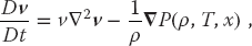
Here, ν is the kinematic viscosity, P is the pressure, and (25.4) gives the derivatives in (25.3) in Cartesian coordinates. This equation describes transfer of the momentum of the fluid within some region of space as a result of forces and flow (think d p/dt = F). There is a simultaneous equation for each of the three velocity components. The v. ∇v term in Dv/Dt describes the transport of momentum in some region of space resulting from the fluid’s flow and is often called the convection or advection term.²⁾ The ∇P term describes the velocity change as a result of pressure changes, and the v∇²v term describes the velocity change resulting from viscous forces (which tend to dampen the flow).

The explicit functional dependence of the pressure on the fluid’s density and temperature P(ρ, T, x) is known as the equation of state of the fluid, and would have to be known before trying to solve the Navier–Stokes equation. To keep our problem simple, we assume that the pressure is independent of density and temperature. This leaves the four simultaneous partial differential equations to solve, (25.1) and (25.3). Because we are interested in steady-state flow around an object, we assume that all time derivatives of the velocity vanish. Because we assume that the fluid is incompressible, the time derivative of the density also vanishes, and (25.1) and (25.3) become

(25.5)

(25.6)

The first equation expresses the equality of inflow and outflow and is known as the condition of incompressibility. In as much as the stream in our problem is much wider than the width (z direction) of the beam, and because we are staying away from the banks, we will ignore the z dependence of the velocity. The explicit PDEs we need to solve then reduce to

(25.7)

(25.8)

(25.9)

25.2.1 Boundary Conditions for Parallel Plates

The plate problem is relatively easy to solve analytically, and so we will do it! This will give us some experience with the equations as well as a check for our numerical solution. To find a unique solution to the PDEs (25.7)–(25.9), we need to specify boundary conditions. As far as we can tell, picking boundary conditions is somewhat of an acquired skill.

We assume that the submerged parallel plates are placed in a stream that is flowing with a constant velocity V₀ in the horizontal direction (Figure 25.1b). If the velocity V₀ is not too high or the kinematic viscosity ν is sufficiently large, then the flow should be smooth and without turbulence. We call such flow laminar. Typically, a fluid undergoing laminar flow moves in smooth paths that do not close on themselves, like the smooth flow of water from a faucet. If we imagine attaching a vector to each element of the fluid, then the path swept out by that vector is called a streamline or line of motion of the fluid. These streamlines can be visualized experimentally by adding colored dye to the stream. We assume that the plates are so thin that the flow remains laminar as it passes around and through them.

If the plates are thin, then the flow upstream of them is not affected, and we can limit our solution space to the rectangular region in Figure 25.2. We assume that the length L and separation H of the plates are small compared to the size of the stream, so the flow returns to uniform as we get far downstream from the plates. As shown in Figure 25.2, there are boundary conditions at the inlet where the fluid enters the solution space, at the outlet where it leaves, and at the stationary plates. In addition, because the plates are far from the stream’s bottom and surface, we assume that the dotted-dashed centerline is a plane of symmetry, with identical flow above and below the plane. We thus have four different types of boundary conditions to impose on our solution:

1. Solid plates   Because there is friction (viscosity) between the fluid and the plate surface, the only way to have laminar flow is to have the fluid’s velocity equal to the plate’s velocity, which means both are zero:
   (25.10)
2. Such being the case, we have smooth flow in which the negligibly thin plates lie along streamlines of the fluid (like a “streamlined” vehicle).
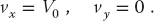
3. Inlet   The fluid enters the integration domain at the inlet with a horizontal velocity V₀. Because the inlet is far upstream from the plates, we assume that the fluid velocity at the inlet is unchanged by the presence of the plates:
   (25.11)
4. Outlet  Fluid leaves the integration domain at the outlet. While it is totally reasonable to assume that the fluid returns to its unperturbed state there, we are not told what that is. So, instead, we assume that there is a physical outlet at the end with the water just shooting out of it. Consequently, we assume that the water pressure equals zero at the outlet (as at the end of a garden hose) and that the velocity does not change in a direction normal to the outlet:
   (25.12)
5. Symmetry plane  If the flow is symmetric about the y = 0 plane, then there cannot be flow through the plane, and the spatial derivatives of the velocity components normal to the plane must vanish:
   (25.13)

This condition follows from the assumption that the plates are along streamlines and that they are negligibly thin. It means that all the streamlines are parallel to the plates as well as to the water surface, and so it must be that v_y = 0 everywhere. The fluid enters in the horizontal direction, the plates do not change the vertical y component of the velocity, and the flow remains symmetric about the centerline. There is a retardation of the flow around the plates because of the viscous nature of the flow and that of the v = 0 boundary layers formed on the plates, but there are no actual v_y components.

Figure 25.2 The boundary conditions for two thin submerged plates. The surrounding box is the integration volume within which we solve the PDEs and upon whose surface we impose the boundary conditions. In practice, the box is much larger than L and H

25.2.2 Finite-Difference Algorithm and Overrelaxation

Now we develop an algorithm for solution of the Navier–Stokes and continuity PDEs using successive over-relaxation. This is a variation of the method used in Chapter 19, to solve Poisson’s equation. We divide space into a rectangular grid with the spacing h in both the x and y directions:

We next express the derivatives in (25.7)–(25.9) as finite differences of the values of the velocities at the grid points using central-difference approximations. For v = 1 m²/s and ρ = 1 kg/m³, this yields

(25.14)

(25.15)

(25.16)

Because v^y ≡ 0 for this problem, we rearrange terms to obtain for v^x:

(25.17)

We recognize in (25.17) an algorithm similar to the one we used in solving Laplace’s equation by relaxation. Indeed, as we did there, we can accelerate the convergence by writing the algorithm with the new value of v^x given as the old value plus a correction (residual):

(25.18)

(25.19)

As performed with the Poisson equation algorithm, successive iterations sweep the interior of the grid, continuously adding in the residual (25.18) until the change becomes smaller than some set level of tolerance, |r_{i, j}| < .

A variation of this method, successive over-relaxation, increases the speed at which the residuals approach zero via an amplifying factor ω:

(25.20)

The standard relaxation algorithm (25.18) is obtained with ω = 1, an accelerated convergence (over-relaxation) is obtained with ω ≥ l, and underrelaxation occurs for ω< 1. Values ω > 2 are found to lead to numerical instabilities. Although a detailed analysis of the algorithm is necessary to predict the optimal value for ω, we suggest that you test different values for ω to see which one provides the fastest convergence for your problem.

25.2.3 Successive Overrelaxation Implementation

1. Modify the program Beam.py, or write your own, to solve the Navier–Stokes equation for the velocity of a fluid in a 2D flow. Represent the x and y components of the velocity by the arrays vx[Nx,Ny] and vy[Nx,Ny].
2. Specialize your solution to the rectangular domain and boundary conditions indicated in Figure 25.2.
3. Use of the following parameter values,
   
   
   leads to the analytic solution
   (25.21)
4. For the relaxation method, output the iteration number and the computed v^x and then compare the analytic and numeric results.
5. Repeat the calculation and see if SOR speeds up the convergence.

25.3 2D Flow over a Beam

Now that the comparison with an analytic solution has shown that our CFD simulation works, we return to determining if the beam in Figure 25.1 might produce a good resting place for salmon. While we have no analytic solution with which to compare, our canoeing and fishing adventures have taught us that standing waves with fish in them are often formed behind rocks in streams, and so we expect there will be a standing wave formed behind the beam.

25.4 Theory: Vorticity Form of Navier–Stokes Equation

We have seen how to solve numerically the hydrodynamics equations

(25.22)

(25.23)

These equations determine the components of a fluid’s velocity, pressure, and density as functions of position. In analogy to electrostatics, where one usually solves for the simpler scalar potential and then takes its gradient to determine the more complicated vector field, we now recast the hydrodynamic equations into forms that permit us to solve two simpler equations for simpler functions, from which the velocity is obtained via a gradient operation.³⁾

We introduce the stream function u(x) from which the velocity is determined by the curl operator:

(25.24)

Note the absence of the z component of velocity v for our problem. Because ∇. ∇×u ≡ 0, we see that any v that can be written as the curl of u automatically satisfies the continuity equation ∇·v = 0. Further, because v for our problem has only x and y components, u(x) needs have only a z component:

(25.25)

It is worth noting that in 2D flows, the contour lines u = constant are the streamlines.

The second simplifying function is the vorticity field w(x), which is related physically and alphabetically to the angular velocity ω of the fluid. Vorticity is defined as the curl of the velocity (sometimes with a – sign):

(25.26)

Because the velocity in our problem does not change in the z direction, we have

(25.27)

Physically, we see that the vorticity is a measure of how much the fluid’s velocity curls or rotates, with the direction of the vorticity determined by the right-hand rule for rotations. In fact, if we could pluck a small element of the fluid into space (so it would not feel the internal strain of the fluid), we would find that it is rotating like a solid with angular velocity ω ∝ w (Lamb, 1993). That being the case, it is useful to think of the vorticity as giving the local value of the fluid’s angular velocity vector. If w = 0, we have irrotational flow.

The field lines of w are continuous and move as if they are attached to the particles of the fluid. A uniformly flowing fluid has vanishing curl, while a nonzero vorticity indicates that the current curls back on itself or rotates. From the definition of the stream function (25.24), we see that the vorticity w is related to it by

(25.28)

where we have used a vector identity for ∇ × (∇ × u). Yet the divergence ∇ • u = 0 because u has a component only in the z-direction and that component is independent of z (or because there is no source for u). We have now obtained the basic relation between the stream function u and the vorticity w:

(25.29)

Equation 25.29 is analogous to Poisson’s equation of electrostatics, ∇²φ = − 4πρ, only now each component of vorticity w is a source for the corresponding component of the stream function u. If the flow is irrotational, that is, if w = 0, then we need only to solve Laplace’s equation for each component of u. Rotational flow, with its coupled nonlinearities equations, leads to more interesting behavior.

As is to be expected from the definition of w, the vorticity form of the Navier–Stokes equation is obtained by taking the curl of the velocity form, that is, by operating on both sides with ∇×. After significant manipulations one obtains

(25.30)

This and (25.29) are the two simultaneous PDEs that we need to solve. In 2D, with u and w having only z components, they are

(25.31)

(25.32)

So after all that work, we end up with two simultaneous, nonlinear, elliptic PDEs that look like a mixture of Poisson’s equation with the wave equation. The equation for u is Poisson’s equation with source w, and must be solved simultaneously with the second. It is this second equation that contains mixed products of the derivatives of u and w and thus introduces the nonlinearity.

25.4.1 Finite Differences and the SOR Algorithm

We solve (25.31) and (25.32) on an N_x × N_y grid of uniform spacing h with

(25.33)

Because the beam is symmetric about its centerline (Figure 25.1a), we need the solution only in the upper half-plane. We apply the now familiar central-difference approximation to the Laplacians of u and w to obtain the difference equation

(25.34)

Likewise, for the product of the first derivatives,

(25.35)

The difference form of the vorticity of the Navier–Stokes equation (25.31) becomes

(25.36)

(25.37)

(25.38)

Note that we have placed u_{i, j} and w_{i, j}, on the LHS of the equations in order to obtain an algorithm appropriate to a solution by relaxation.

The parameter R in (25.38) is related to the Reynolds number. When we solve the problem in natural units, we measure distances in units of grid spacing h, velocities in units of initial velocity V₀, stream functions in units of V₀h, and vorticity in units of V₀/h. The second form is in regular units and is dimensionless. This R is known as the grid Reynolds number and differs from the physical R, which has a pipe diameter in place of the grid spacing h.

The grid Reynolds number is a measure of the strength of the coupling of the nonlinear terms in the equation. When the physical R is small, the viscosity acts as a frictional force that damps out fluctuations and keeps the flow smooth. When R is large (R 2000), physical fluids undergo phase transitions from laminar to turbulent flow in which turbulence occurs at a cascading set of smaller and smaller space scales (Reynolds, 1883). However, simulations that produce the onset of turbulence have been a research problem because Reynolds first experiments in 1883 (Falkovich and Sreenivasan, 2006), possibly because the laminar flow is stable against small perturbations and some large-scale “kick” may be needed to change laminar to turbulent flow. Recent research along these lines have been able to find unstable, traveling-wave solutions to the Navier–Stokes equations, and the hope is that these may lead to a turbulent transition (Fitzgerald, 2004).

As discussed in Section 25.2.2, the finite-difference algorithm can have its convergence accelerated by the use of successive over-relaxation (25.36):

(25.39)

Here, ω is the over-relaxation parameter and should lie in the range 0 < ω < 2 for stability. The residuals are just the changes in a single step, r⁽¹⁾ = u^new − u^old and r⁽²⁾ = w^new − w^old:

(25.40)

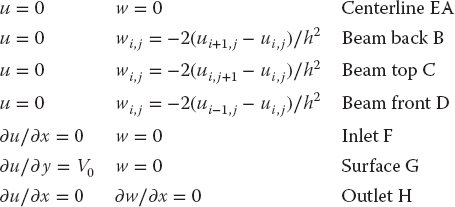
25.4.2 Boundary Conditions for a Beam

A well-defined solution of these elliptic PDEs requires a combination of (less than obvious) boundary conditions on u and w. Consider Figure 25.3, based on the analysis of Koonin (1986). We assume that the inlet, outlet, and surface are far from the beam, which may not be evident from the not-to-scale figure.

1. Freeflow If there were no beam in the stream, then we would have free flow with the entire fluid possessing the inlet velocity:
   (25.41)

   

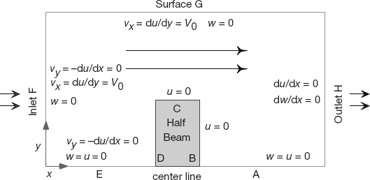
   Figure 25.3 Boundary conditions for flow around the beam in Figure 25.1. The flow is symmetric about the centerline, and the beam has length L in the x direction (along flow).

   1. (Recall that we can think of w = 0 as indicating no fluid rotation.) The center-line divides the system along a symmetry plane with identical flow above and below it. If the velocity is symmetric about the centerline, then its y component must vanish there:
   (25.42)
2. Centerline The centerline is a streamline with u = constant because there is no velocity component perpendicular to it. We set u = 0 according to (25.41). Because there cannot be any fluid flowing into or out of the beam, the normal component of velocity must vanish along the beam surfaces. Consequently, the streamline u = 0 is the entire lower part of Figure 25.3, that is, the center-line and the beam surfaces. Likewise, the symmetry of the problem permits us to set the vorticity w = 0 along the centerline.
3. Inlet At the inlet, the fluid flow is horizontal with uniform x component V₀ at all heights and with no rotation:
   (25.43)
4. Surface We are told that the beam is sufficiently submerged so as not to disturb the flow on the surface of the stream. Accordingly, we have free-flow conditions on the surface:
   (25.44)
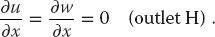
5. Outlet Unless something truly drastic happens, the conditions on the far downstream outlet have little effect on the far upstream flow. A convenient choice is to require the stream function and vorticity to be constant:
   (25.45)
6. Beamsides We have already noted that the normal component of velocity v_x and stream function u vanish along the beam surfaces. In addition, because the flow is viscous, it is also true that the fluid “sticks” to the beam somewhat and so the tangential velocity also vanishes along the beam’s surfaces. While these may all be true conclusions regarding the flow, specifying them as boundary conditions would over-restrict the solution (see Table 19.2 for elliptic equations) to the point where no solution may exist. Accordingly, we simply impose the no-slip boundary condition on the vorticity w. Consider a grid point (x, y) on the upper surface of the beam. The stream function u at a point (x, y + h) above it can be related via a Taylor series in y:
   (25.46)
7. Because w has only a z component, it has a simple relation to ∇ × ν:
   (25.47)
8. Because of the fluid’s viscosity, the velocity is stationary along the beam top:
   (25.48)
9. Because the current flows smoothly along the top of the beam, v_y must also vanish. In addition, because there is no x variation, we have
   (25.49)
10. After substituting these relations into the Taylor series (25.46), we can solve for w and obtain the finite-difference version of the top boundary condition:
    (25.50)
11. Similar treatments applied to other surfaces yield the boundary conditions.
    (25.51)

25.4.3 SOR on a Grid

Beam.py in Listing 25.1 is our program for the solution of the vorticity form of the Navier–Stokes equation. You will notice that while the relaxation algorithm is rather simple, some care is needed in implementing many boundary conditions. Relaxation of the stream function and of the vorticity are performed by separate functions.

Listing 25.1 Beam.py solves the Navier–Stokes equation for the flow over a plate.

25.4.4 Flow Assessment

1. Use Beam.py as a basis for your solution for the stream function u and the vorticity w using the finite-differences algorithm (25.36).
2. A good place to start your simulation is with a beam of size L = 8h, H = h, Reynolds number R = 0.1, and intake velocity V₀ = 1. Keep your grid small during debugging, say, N_x = 24 and N_y = 70.
3. Explore the convergence of the algorithm.
   1. a) Print out the iteration number and u values upstream from, above, and downstream from the beam.
   2. b) Determine the number of iterations necessary to obtain three-place convergence for successive relaxation (ω = 0).
   3. c) Determine the number of iterations necessary to obtain three-place convergence for successive over-relaxation (ω 0.3). Use this number for future calculations.
4. Change the beam’s horizontal placement so that you can see the undisturbed current entering on the left and then developing into a standing wave. Note that you may need to increase the size of your simulation volume to see the effect of all the boundary conditions.
5. Make surface plots including contours of the stream function u and the vorticity w. Explain the behavior seen.
6. Is there a region where a big fish can rest behind the beam?
7. The results of the simulation (Figure 25.4) are for the one-component stream function u. Make several visualizations showing the fluid velocity throughout the simulation region. Note that the velocity is a vector with two components (or a magnitude and direction), and both degrees of freedom are interesting to visualize. A plot of vectors would work well here.

   

   Figure 25.4 Two visualizations of the stream function u for Reynold’s number R = 5. The one on the left uses contours, while the one on the right uses color.

   

   Figure 25.5 (a) The velocity field around the beam as represented by vectors. (b) The vorticity as a function of x and y for the same velocity field. Rotation is seen to be largest behind the beam.

8. Explore how increasing the Reynolds number R changes the flow pattern. Start at R = 0 and gradually increase R while watching for numeric instabilities. To overcome the instabilities, reduce the size of the relaxation parameter ω and continue to larger R values.
9. Verify that the flow around the beam is smooth for small R values, but that it separates from the back edge for large R, at which point a small vortex develops, as can be seen in Figure 25.5.

25.4.5 Exploration

1. Determine the flow behind a circular rock in the stream.
2. The boundary condition at an outlet far downstream should not have much effect on the simulation. Explore the use of other boundary conditions there.
3. Determine the pressure variation around the beam.

1) We acknowledge some helpful reading of by Satoru S. Kano.

2) We discuss pure advection in Section 24.1. In oceanology or meteorology, convection implies the transfer of mass in the vertical direction where it overcomes gravity, whereas advection refers to transfer in the horizontal direction.

3) If we had to solve only the simpler problem of irrotational flow (no turbulence), then we would be able to use a scalar velocity potential, in close analogy to electrostatics (Lamb, 1993). For the more general rotational flow, two vector potentials are required.