Appendix

1.Basic facts from real analysis

(More details can be found in the standard literature.1) The euclidian norm (or geometric length) of a vector x ∈ ℝⁿ with components x_j, is

The ball with center x and radius r is the set

A subset S ⊆ ℝⁿ is closed if each convergent sequence of elements x_k ∈ S has its the limit point x is also in S:

The set S is open if its complement ℝⁿ \ S is closed. The following statements are equivalent:

(O′) S is open.

(O″) For each x ∈ S there is some r > 0 such that B_r(x) ⊆ S.

The set S is bounded if S ⊆ B_r(0) holds for some r ≥ 0. S is said to be compact if S is bounded and closed.

LEMMA A.2 (HEINE–BOREL). S ⊆ ℝⁿ is compact if and only if

 

(HB)	every family of open sets O ⊆ ℝn such that every x ∈ S lies in at least one O ∈ , admits a finite number of sets O1 , . . . , O ∈ with the covering property

It is important to note that compactness is preserved under forming direct products:

•If X ⊆ ℝⁿ and Y ⊆ ℝ^m are compact sets, then X × Y ⊆ ℝ^n+m is compact.

Continuity. A function f : S → ℝ^m is continuous if for all convergent sequences of elements x_k ∈ S, the sequence of function values f(x_k) converges to the value of the limit:

The following statements are equivalent:

 

(C′)	f : S → ℝm is continuous.
(C″)	For each open set O ⊆ ℝm, there exists an open set O′ ⊆ ℝn such that i.e., the inverse image f−1(O) is open relative to S.
(C″′)	For each closed set C ⊆ ℝm, there exists a closed set C′ ⊆ ℝn such that i.e., the inverse image f−1(C)is closed relative to S.

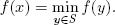
LEMMA A.3 (Extreme values). If the real-valued function f : S → ℝ is continuous on the nonempty compact set S ⊆ ℝⁿ, then there exist elements x_*, x^* ∈ S such that

Differentiability. The function f : S → ℝ is differentiable on the open set S ⊆ ℝⁿ if for each x ∈ S there is a (row) vector ∇f(x) such that for every d ∈ ℝⁿ of unit length ||d|| = 1, one has

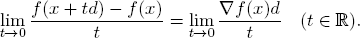
∇f(x) is the gradient of f. Its components are the partial derivatives of f:

NOTA BENE. All differentiable functions are continuous — but not all continuous functions are differentiable.

2.Convexity

A linear combination of elements x₁, . . . , x_m is an expression of the form

where λ₁, . . . , λ_m are scalars (real or complex numbers). The linear combination z with scalars λ_i is affine if

An affine combination is a convex combination if all scalars λ_i are nonnegative real numbers. The vector λ = (λ₁, . . . , λ_m) of the m scalars λ_i of a convex combination is a probability distribution on the index set

Convex sets. The set S ⊆ ℝⁿ is convex if it contains with every x, y ∈ S also the connecting line segment:

It is easy to verify:

•The intersection of convex sets yields a convex set.

•The direct product S = X × Y ⊆ ℝ^n×m of convex sets X ⊆ ℝⁿ and Y ⊆ ℝ^m is a convex set.

EX. A.9 (Probability distributions). For X = {1, . . . , n}, the set

of all probability distributions on X is convex. Because the function

is continuous, the set

is closed. The collection of nonnegative vectors is closed in ℝⁿ. Since the intersection of closed sets is closed, one deduces that

is closed and bounded and thus compact.

Convex functions. A function f : S → ℝ is convex (up) on the convex set S if for all x, y ∈ S and for all scalars 0 ≤ λ ≤ 1,

This definition is equivalent to the requirement that one has for any finitely many elements x₁, . . . , x_m ∈ S and probability distributions {λ₁, . . . , λ_m),

The function f is concave (or convex down) if g = −f is convex (up).

A differentiable function f : S → ℝ on the open set S ⊆ ℝⁿ is convex (up) if and only if

Assume, for example, that ∇f(x)(y – x) ≥ 0 it true for all y ∈ S, then one has

On the other hand, if ∇f(x)(y – x) < 0 is true for some y ∈ S, one can move from x a bit into the direction of y and find an element x′ with f(x′) < f(x). Hence one has a criterion for minimizers of f on S:

LEMMA A.4. If f is a differentiable convex function on the convex set S, then for any x ∈ S, the statements are equivalent:

(1)

(2)∇f(x)(y – x) ≥ 0 for all y ∈ S.

If strict inequality holds in (76) for all y ≠ x, f is said to be stricly convex.

In the case n = 1 (i.e., S ⊆ ℝ), a simple criterion applies to twice differentiable functions:

For example, the logarithm function f(x) = ln x is seen to be strictly concave on the open interval S = (0, ∞) because of

3.Polyhedra and linear inequalities

A polyhedron is the solution set of a finite system of linear equalities and inequalities. More precisely, if A ⊆ ℝ^m×n is a matrix and b ∈ ℝ^m a parameter vector, then the (possibly empty) set

is a polyhedron. Since the function x ↦ Ax is linear (and hence continuous), one immediately checks that P(A, b) is a closed convex subset of ℝⁿ. Often, nonnegative solutions are of interest and one considers the associated polyhedron

with the identity matrix I ∈ ℝ^n×n.

EX. A.10. The set (X) of all probability distributions on the finite set X is a polyhedron. (cf. Ex. A.9.)

LEMMA A.5 (FARKAS2). If P(A, b) ≠ ∅, then for any c ∈ ℝⁿ and z ∈ ℝ, the following statements are equivalent:

(1)c^Tx ≤ z holds for all x ∈ P(A, b).

(2)There exists some y ≥ 0 such that y^TA = c^T and y^Tb ≤ z.

Lemma A.5 is a direct consequence of the algorithm of FOURIER,³ which generalizes the Gaussian elimination method from systems of linear equalities to general linear inequalities.⁴

The formulation of Lemma A.5 is one version of several equivalent characterizations of the solvability of finite linear (in)equality systems, known under the comprehensive label FARKAS Lemma. A nonnegative version of the FARKAS Lemma is:

LEMMA A.5 (FARKAS+). If P₊ (A, b) ≠ Ø, then for any c ∈ ℝⁿ and z ∈ ℝ, the following statements are equivalent:

(1)c^Tx ≤ z holds for all x ∈ P₊(A, b).

(2)There exists some y ≥ 0 such that y^TA ≥ c^T and y^Tb ≤ z.

EX. A.11. Show that Lemma A.5 and Lemma A.6 are equivalent.
Hint: Every x ∈ ℝⁿ is a difference x = x⁺ − x⁻ of two nonnegative vectors x⁺, x⁻. So

4.BROUWER’s fixed-point theorem

A fixed-point of a map f : X → X is a point x ∈ X such that f(x) = x. It is usually difficult to find a fixed-point (or even to decide whether a fixed-point exists). Well-known sufficient conditions were formulated by BROUWER5:

THEOREM A.2 (BROUWER). Let X ⊆ ℝⁿ be a convex, compact and non-empty set and f : X → X a continuous function. Then f has a fixed-point.

Proof. See, e.g., the enyclopedic text of GRANAS and DUGUNDJI [22].

For game-theoretic applications, the following implication is of interest.

CORROLLARY A.1. Let X ⊆ ℝⁿ be a convex, compact and nonempty set and G : X × X → ℝ a continuous map that is concave in the second variable, i.e.,

 

(C)	for every x ∈ X, the map y ↦ G(x, y) is concave.

Then there exists a point x^* ∈ X such that for all y ∈ X, one has

Proof. One derives a contradiction from the supposition that the Corollary is false. Indeed, if there is no x^* with the claimed property, then each x ∈ X lies in at least one of the sets

Since G is continuous, the sets O(y) are open. Hence, as X is compact, already finitely many cover all of X, say

For all x ∈ X, define the parameters

x lies in at least one of the sets O(y). Therefore, we have

Consider now the function

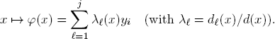
Since G is continuous, also the functions x ↦ d(x) are continuous. Therefore, φ : X → X is continuous. By BROUWER’s Theorem A.2, φ has a fixed-point

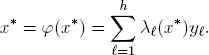
Since G(x, y) is concave in y and x^* is an affine linear combination of the y, we have

If the Corollary were false, one would have

for each summand and, in at least one case, even a strict inequality

which would produce the contradictory statement

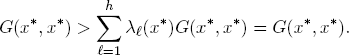
It follows that the Corollary must be correct.

5.The MONGE algorithm

The MONGE algorithm with respect to coefficient vectors c, υ ∈ ℝⁿ has two versions.

The primal MONGE algorithm constructs a vector x(υ) with the components

The dual MONGE algorithm constructs a vector y(c) with the components

Notice:

The important property to observe is as follows:

LEMMA A.7. The MONGE vectors x(υ) and y(c) yield the equality

Proof. Writing x = x(υ) and y = y(c), notice for all 1 ≤ k, ≤ n,

and hence

6.Entropy and BOLTZMANN distributions

6.1.BOLTZMANN distributions

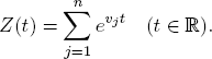
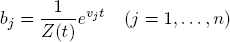
The partition function Z for a given vector υ = (υ₁, υ_n) of real numbers υ_j takes the (strictly positive) values

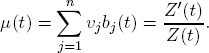
The associated BOLTZMANN probability distribution b(t) has the components

and yields the expected value function

The variance of υ is its expected quadratic deviation from μ(t):

One has σ²(t) ≠ 0 unless all υ_j are equal to a constant K (and hence μ(t) = K for all t). Because μ′(t) = σ²(t) > 0, one concludes that μ(t) is strictly increasing in t unless μ(t) is constant.

Arrange the components of υ such that υ₁ ≤ υ₂ ≤ . . . ≤ υ_n. Then

which implies b_j(t) → 0 if υ_j < υ_n. It follows that the limit distribution b(∞) is the uniform distribution on the maximizers of υ. Similarly, one has

and concludes that the limit distribution b(−∞) is the uniform distribution on the minimizers of υ.

THEOREM A.3. For every value υ₁ < ξ < υ_n, there is a unique parameter t such that

Proof. The expected value function μ(t) is strictly monotone and continuous on ℝ and satisfies

So, for every prescribed value ξ between the extrema υ₁ and υ_n, there must exist precisely one t with μ(t) = ξ.

6.2.Entropy

The real function h(x) = x ln x is defined for all nonnegative real numbers6 and has the strictly increasing derivative

So h is strictly convex and satisfies the inequality

h is extended to nonnegative real vectors x = (x₁, . . . , x_n) via

The strict convexity of h becomes the inequality

with the gradient

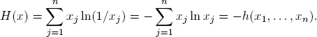
In the case x₁ + . . . + x_n = 1, the nonnegative vector x is a probability distribution on the set {1, . . . , n} and has7 the entropy

We want to show that BOLTZMANN probability distributions are precisely the ones with maximal entropy relative to given expected values.

THEOREM A.4. Let υ = (υ₁, . . . , υ_n) be a vector of real numbers and b the BOLTZMANN distribution on {1, . . . , n} with components

with respect to some t. Let p = (p₁, . . . , p_n) be a probability distribution with the same expected value

Then one has either p = b or H(p) < H(b).

Proof. For d = p − b, we have ∑_j d_j = ∑_j p_j − ∑_j b_j = 1 – 1 = 0, and therefore

In the case p ≠ b, the strict convexity of h thus yields

LEMMA A.8 (Divergence). Let a₁, . . . , a_n, p₁, . . . , p_n be arbitrary nonnegative numbers. Then

Equality is attained exactly when a_i = p_i holds for all i = 1, . . . , n.

Proof. We may assume p_i ≠ 0 for all i and make use of the well-known fact (which follows easily from the concavity of the logarithm function):

Then we observe

and therefore

Equality can only hold if ln(a_i/p_i) = (a_i/p_i) – 1, and hence a_i = p_i is true for all i.

7.MARKOV chains

A (discrete) MARKOV chain8 on a finite set X is a (possibly infinite) random walk on the graph G = G(X) whose edges (x, y) are labeled with probabilities 0 ≤ p_xy ≤ 1 such that

The walk starts in some node s ∈ X and then iterates subsequent transitions x → y with probabilities p_xy:

Let P = [p_xy] be the matrix of transition probabilities and Pⁿ = the n-fold matrix product of P. Then the random walk has reached the node y after n iterations with probability

In other words: The x₀-row of Pⁿ is a probability distribution p⁽ⁿ⁾ on X.

The MARKOV chain is connected if every node in G can be reached from any other node with non-zero probability in a finite number of transitional steps. This means:

•There exists some natural number m such that > 0 holds for all x, y ∈ X.

LEMMA A.9. If the MARKOV chain is connected and p_xx > 0 holds for at least one x ∈ X, then the MARKOV chain converges in the following sense:

(1)The limit matrix exists.

(2)P^∞ has identical row vectors p^(∞).

(3)As a row vector, p^(∞) is the unique solution of the (in)equality system

A useful sufficient condition for the computation of a limit distribution p^(∞) of a MARKOV chain is given in the next example.

EX. A.12. Let P = [p_xy] ∈ ℝ^X×X be a MARKOV transition probability matrix and p ∈ ℝ^X a probability distribution on X such that

Then P^Tp = p holds. Indeed, one computes for each x ∈ X:

 

 

 

_____________________________

1 e.g., RUDIN [39].

² GY. FARKAS (1847–1930).

³ J. FOURIER (1768–1830).

⁴ See, e.g., Section 2.4 in FAIGLE et al. [17].

⁵ L. E. J. BROUWER (1881–1966).

⁶ With the understanding ln 0 = −∞ and 0 · ln 0 = 0.

⁷ By definition!

⁸ For more details, see, e.g., KEMENY and SNELL [25].