Chapter 4
Investing and Betting
The opponent of a gambler is usually a player with no specific optimization goal. The opponent’s strategy choices seem to be determined by chance. Therefore, the gambler will have to decide on strategies with good expected returns. Information plays an important role in the quest for the best decision. Hence the problem how to model information exchange and common knowledge among (possibly more than two) players deserves to be addressed as well.
Assume that an investor (or bettor or gambler or simply player) is considering a financial engagement in a certain venture. Then the obvious — albeit rather vague — big question for the investor is:
•What decision should best be taken?
More specifically, the investor wants to decide whether an engagement is worthwhile at all and, if so, how much of the available capital should be invested how. Obviously, the answer depends on additional information: What is the likelihood of a success? What gain can be expected? What is the risk of a loss? etc.
The investor is thus about to participate as a player in a 2-person game with an opponent whose strategies and objective are not always clear or known in advance. Relevant information is not completely (or not reliably) available to the investor so that the decision must be made under uncertainties. Typical examples are gambling and betting where the success of the engagement depends on events that may or may not occur and hence on “fortune” or “chance”. But also investments in the stock market fall into this category when it is not clear in advance whether the value of a particular investment will rise or fall.
We are not able to answer the big question above completely but will discuss various aspects of it. Before going into further details, let us illustrate the difficulties of the subject with a classical — and seemingly paradoxical — gambling situation.
The St. Petersburg paradox. Imagine yourself as a potential player in the following game of chance.
EX. 4.1 (St. Petersburg game). A coin (with faces “H” and “T”) is tossed repeatedly until “H” shows. If this happens at the nth toss, a participating player will receive αn = 2n euros. There is a participation fee of a0 euros, however. So the net gain of the player is

if the game stops at the nth toss. At what entrance fee a0 would a participation in the game be attractive?
Assuming a fair coin in the St. Petersburg game, the probability to go through more than n tosses (and hence to have the first n results as “T”) is

So the game ends almost certainly after a finite number of tosses. The expected return to a participant is nevertheless infinite:
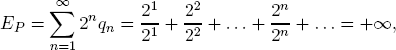
which might suggest that a player should be willing to pay any finite amount a0 for being allowed into the game. In practice, however, this could be a risky venture (see Ex. 4.2).
EX. 4.2. Show that the probability of receiving a return of 100 euros or more in the St. Petersburg game is less than 1%. So a participation fee of a0 = 100 euros or more appears to be not attractive because it will not be recovered with a probability of more than 99%.
Paradoxically, when we evaluate the utility of the return αn = 2n not directly but by its logarithm log2 αn = log2 2n = n, the St. Petersburg payoff has a finite utility expectation:
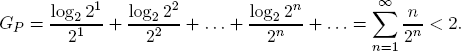
This observation suggests that one should expect an utility value of less than 2 and hence a return of less than 22 = 4 euros.
REMARK 4.1 (Logarithmic utilities). The logarithm function as a measure for the utility value of a financial gain was introduced by D. BERNOULLI1 in his analysis of the St. Petersburg game. This concave function plays an important role in our analysis as well.
Whether one uses log2 x, the logarithm base 2, or the natural logarithm ln x does not make an essential difference since the two functions differ just by a scaling factor:

Arithmetic and geometric growth. If investments are repeated, the question arises how to evaluate the evolution of the capital arising from the investments. To make this question more precise, assume that a capital of initial size b0 takes on the values
in discrete time steps. The arithmetic growth rate up to time t is the number
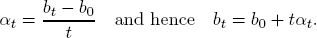
The geometric growth rate up to time t is the number

Passing to logarithms, the geometric growth rate becomes the logarithmic geometric growth rate

which is the arithmetic growth rate of the logarithmic utility. Since x ↦ ln x is a monotonically strictly increasing function, optimizing γt is equivalent with optimizing of Gt. In other words:
Optimizing the geometric growth rate is equivalent with optimizing the arithmetic growth rate of the logarithmic utility.
1.Proportional investing
Our general model consists of a potential investor with an initial portfolio B of b > 0 euros (or dollars or...) and an investment opportunity A. If things go well, an investment of size x would bring a return rx > x. If things do not go well, the investment will return nothing.
In the analysis, we will denote the net return rate by

The investor is to decide what portion of B should be invested. The investor believes:
| (PI) |
Things go well with probability p > 0 and do not go well with probability q = 1 − p. |
1.1.Expected portfolio
Under the assumption (PI), the investor’s expected portfolio value after the investment x is

since an amount of size b − x is not invested and therefore not at risk. The derivative is

So B(x) is strictly increasing if ρ > q/p and non-increasing otherwise. Hence, if the investor’s decision is motivated by the maximization of the expected portfolio value B(x), the naive investment rule applies:
| (NIR) |
If ρ > q/p, invest all of B in A and expect the return |

|
| |
If ρ ≤ q/p, invest nothing since no proper gain is expected. |
In spite of its intuitive appeal, rule (NIR) can be quite risky (see Ex. 4.3).
EX. 4.3. Assume that the investment opportunity A offers the return rate r = 100 for an investment in the case it goes well. Assume further that an investor estimates the probability for A to go well to be p = 10%. In view of

a naive investor would invest the full amount x* = b and expect a tenfold return:

However, with probability q = 90%, the investment should be expected to result in a total loss.
1.2.Expected utility
With respect to the logarithmic utility function ln x, the expected utility of an investment of size x with net return rate ρ would be

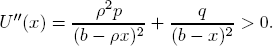
The marginal utility of x is the value of the derivative

The second derivative is
So the investment x* has optimal (logarithmic) utility if

EX. 4.4. In the situation of Ex. 4.3, one has

with the derivative

U′(x*) = 0 implies x* = b/11. Hence the portion a* = 1/11 of the portfolio should be invested in order to maximize the expected utility U. The rest of the portfolio should be retained and not be invested.
The expected value of the portfolio with respect to x* = b/11 is

and thus much lower than under the naive investment policy. However, the investor is guaranteed to preserve at least 10/11 of the original portfolio value.
1.3.The fortune formula
Let a = x/b denote the fraction of the portfolio B to be possibly invested into the opportunity A with r-fold return if A works out. With ρ = r − 1 > 0, the expected logarithmic utility function then becomes

with the derivative

If a loss is to be expected with positive probability q > 0, and the investor decides on a full investment, i.e.,chooses a = 1, then the expected utility (value)

results — no matter how big the net return rate ρ might be.
On the other hand, the choice a = 0 of no investment has the utility

The investment fraction a* yielding the optimal utility lies somewhere between these extremes.
LEMMA 4.1 Let u′(a) be as in (36) and 0 < a* < 1. Then

Proof. Exercise left to the reader.
The choice of the investment rate a* with optimal expected logarithmic utility u(a*) yields the so-called fortune formula of KELLY [24]:
An investment strategy according to (37) is known as a G-strategy or KELLY strategy.2
Betting one’s belief. It is important to keep in mind that the probability p in the fortune formula (37) is the subjective evaluation of an investment success by the investor.
The “true” probability is often unknown at the time of the investment. However, if p reflects the investor’s best knowledge about the true probability, there is nothing better the investor could do. This truism is known as the investment advice
Bet your belief !
2.Fair odds
An investment into an opportunity A offering a return of r ≥ 1 euros per euro invested with a certain probability Pr(A) or returning nothing (with probability 1 − Pr(A)) is called a bet on A. The investor is then a bettor (or a gambler) and the net return

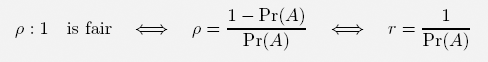
is the payoff of the bet. The payoff is assumed to be guaranteed by a bookmaker (or bank). The net return rate is also denoted3 by ρ : 1 and known as the odds of the bet.
The expected gain (per euro) of the gambler, and hence the bookmaker’s loss, is

The odds ρ : 1 are considered to be fair if the gambler and the bookmaker have the same expected gain, i.e., if

holds. In other words:
If the true probability Pr(A) is not known to the bettor, it needs to be estimated. Suppose the bettor’s estimate for Pr(A) is p. Then the bet appears (subjectively) advantageous if and only if

The bettor will consider the odds ρ : 1 as fair if

In the case E(p) < 0, of course, the bettor would not expect a gain but a loss on the bet — on the basis of the information that has led to the subjective probability estimate p for Pr(A).
Examples. Let us look at some examples.
EX. 4.5 (DE MÉRÉ’s game4). Let A be the event that no “6” shows if a single 6-sided die is rolled four times. Suppose the odds 1 : 1 are offered on A. If the gambler considers all results as equally likely, the gambler’s estimate of the probability for A is

because there are 64 = 1296 possible result sequences on 4 rolls of the die, of which 54 = 625 correspond to A. So the player should expect a negative return:

In contrast, let à be the event that no double 6 shows if a pair of dice is rolled 24 times. Now the prospective gambler estimates Pr(Ã) as

Consequently, the odds 1 : 1 on à would lead the gambler to expect a proper gain:

EX. 4.6 (Roulette). Let W = {0, 1, 2, . . . , 36} represent a roulette wheel and assume that 0 ∈ W is colored green while eighteen numbers in W are red and the remaining eighteen numbers black. Assume that a number X ∈ W is randomly determined by spinning the wheel and allowing a ball come to rest at one of these numbers.
| (a) |
Fix w ∈ W and the gross return rate r = 18 on the event |
| |
|
| |
Should a gambler expect a positive gain when placing a bet on Aw? |
| (b) |
Suppose the bank offers the odds 1 : 1 on the event R = {X = red}. Should a gambler consider these odds on R to be fair? |
The doubling strategy. For the game of roulette (see Ex. 4.6) and for similar betting games with odds 1 : 1 (i.e., with the return rate r = 2) a popular wisdom5 recommends repeated betting according to the following strategy:
| (D) |
Bet the amount 1 on R = {X = red}. If R does not occur, continue with the double amount 2 on R. If R does not show, double again and bet 4 on R and so on — until the event R happens. |
Once R shows, one has a net gain of 1 on the original investment of size 1 (see Ex. 4.7). The probability for R not to happen in one spin is 19/37. So the probability of seeing red in one of the first n spins of an equally balanced roulette wheel is high:

Hence: Strategy (D) achieves a net gain of 1 with high probability.
Paradoxically(?), the expected net gain for betting any amount x > 0 on the event R is always strictly negative however:

EX. 4.7. Show for the game of roulette with a well-balanced wheel:
| (1) |
If {X = red} shows on the fifth spin of the wheel only, strategy (D) has lost a total of 15 on the first 4 spins. However, having invested 16 more and then winning 25 = 32 on the fifth spin, yields the overall net return |
| |

|
| (2) |
The probability for {X = red} to happen on the first 5 spins is more than 95%. |
REMARK 4.2. The problem with strategy (D) is its risk management. A player has only a limited amount of money available in practice. If the player wants to limit the risk of a loss to B euros, then the number of iterations in the betting sequence is limited to at most k, where

Consequently:
•The available budget B is lost with probability (19/37)k.
•The portfolio grows to B + 1 with probability 1 − (19/37)k.
3.Betting on alternatives
Consider k mutually exclusive events A0, A1, . . . , Ak−1 of which one will occur with certainty and a bank that offers the odds ρi : 1 for bets on the k events Ai, which means:
| (1) |
The bank guarantees a total payoff of ri = ρi + 1 euros for each euro invested in Ai if the event Ai occurs. |
| (2) |
The bank offers a scenario with 1/ri being the probability for Ai to occur. |
Suppose a gambler estimates the events Ai to occur with probabilities pi and decides to invest the capital B of unit size6 b = 1 fully. Under this condition, a (betting) strategy is a k-tuple a = (a0, a1, . . . , ak−1) of numbers ai ≥ 0 such that

with the interpretation that the portion ai of the capital will be bet onto the occurrence of event Ai for i = 0, 1, . . . , k − 1. The gambler’s expected logarithmic utility of strategy a is
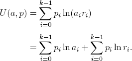
Notice that p = (p0, p1, . . . , pk−1) is a strategy in its own right and that the second sum term in the expression for U(a, p) does not depend on the choice of a. So only the first sum term is of interest when the gambler seeks a strategy with optimal expected utility.
THEOREM 4.1. Let p = (p0, p1, . . . , pk−1) be the gambler’s probability assessment. Then:
Consequently, a* = p is the strategy with the optimal logarithmic utility under the gambler’s expectations.
Proof. The function f(x) = x − 1 − ln x is defined for all x > 0. Its derivative

is negative for x < 1 and positive for x > 1. So f(x) is strictly decreasing for x < 1 and strictly increasing for x > 1 with the unique minimum f(1) = 0. This yields BERNOULLI’s inequality

Applying the BERNOULLI inequality, we find

with equality if and only if ai = pi for all i = 0, 1, . . . k1.

Theorem 4.1 leads to the betting rule with the optimal expected logarithmic utility:
| (BR) |
For all i = 0, 1, . . . , k − 1, bet the portion  of the capital B on the event Ai. of the capital B on the event Ai. |
REMARK 4.3. The proportional rule (BR) depends only on the gambler’s probability estimate p. It is independent of the particular odds ρi : 1 the bank may offer!
Fair odds. As in the proof of Theorem 4.1, one sees:

with equality if and only if ri = 1/pi holds for all i = 0, 1, . . . , k − 1. It follows that the best odds ρi : 1 for the bank (and worst for the gambler) are given when

In this case, the gambler expects the logarithmic utility of the optimal strategy p as

We understand the odds as in (40) to be fair in the context of betting with alternatives.
3.1.Statistical frequencies
Assume that the gambler of the previous sections has observed:
•The event Ai has popped up si times in n consecutive instances of the bet.
So, under the strategy a, the original portfolio B of unit size b = 1 would have developed into size

with the logarithmic utility
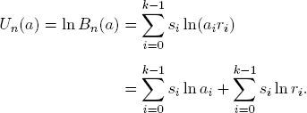
As in the proof of Theorem 4.1, the gambler finds in hindsight:
COROLLARY 4.1. The strategy a* = (s0/n, . . . , sk−1/n) would have led to the maximal logarithmic utility value
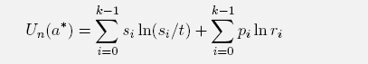
and hence to the growth with the maximal geometric growth rate

Based on the observed frequencies si the gambler might reasonably estimate the events Ai to occur with probabilities according to the relative frequencies

and then expect optimal geometric growth.
4.Betting and information
Assuming a betting situation with the k alternatives A0, A1, . . . , Ak−1 and the odds ρx : 1 (for x = 0, 1, . . . , k − 1) as before, suppose, however, that the event Ax is actually already established — but that the bettor does not have this information before placing the bet.
Suppose further that information now arrives through some (human or technical) communication channel K so that the outcome Ax is reported to the bettor (perhaps incorrectly) as Ay:
The question is:
•Having received the (“insider”) information “y”, how should the bettor place the bet?
To answer this question, let
p(x|y) = probability for the true result to be x when y is received.
REMARK 4.4. The parameters p(x|y) are typically subjective evaluations of the bettor’s trust in the channel K.
A betting strategy in this setting of information transmission becomes a (k × k)-matrix A with coefficients a(x|y) ≥ 0 which satisfy

According to strategy A, a(x|y) would be the fraction of the budget that is bet on the event Ax when y is received. In particular, the bettor’s trust matrix P with the coefficients p(x|y) is a strategy. In the case where Ax is the true result, one therefore expects the logarithmic utility

As in Corollary 4.1, we find for all x = 0, 1, . . . , k − 1:

So the trust matrix P yields also an optimal strategy (under the given trust in K on part of the bettor) and confirms the betting rule:
Information transmission. Let p = (x0, x1, . . . , xk−1) be the bettor’s probability estimates on the k events A0, A1, . . . , Ak−1 or, equivalently, on the index set {0, 1, . . . , k − 1}. Then the expected logarithmic utility of strategy A is relative to base 2:
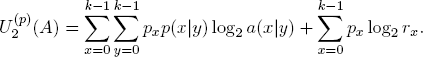
NOTA BENE. The probabilities px are estimates on the likelihood of the events Ax, while the probabilities p(x|y) are estimates on the trust into the reliability of the communication channel K. They are logically not related.
Setting

we thus have

where

is the increase of the bettor’s expected logarithmic utility due to the communication via channel K.
REMARK 4.5 (Channel capacity). Given the channel K as above with transmission (trust) probabilities p(s|r) and the probability distribution

on the channel inputs x, the parameter T(X, Y) is the (information) transmission rate of K.
Maximizing over all possible input distributions p, one obtains the channel capacity C(K) as the smallest upper bound on the achievable transmission rates:
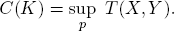
The parameter C(K) plays an important role in the theory of information and communication in general.7
EX. 4.8. A bettor expects the event A0 with probability 80% and the alternative event A1 with probability 20%. What bet should be placed?
Suppose now that an expert tells the bettor that A1 is certain to happen. What bet should the bettor place under the assumption that the expert is right with probability 90%?
5.Common knowledge
Having discussed information with respect to betting, let us digress a little and take a more general view on information and knowledge.8 Given a system  , we ask:
To what extent does common knowledge in a group of agents influence individual conclusions about the state of ?
To explain more concretely what is meant here, we first discuss a well-known riddle.
5.1.Red and white hats
Imagine the following situation:
| (I) |
Three girls, G1, G2 and G3, with red hats sit in a circle. |
| (II) |
Each girl knows that their hats are either red or white. |
| (III) |
Each girl can see the color of all hats except her own. |
Now the teacher comes and announces:
| (1) |
There is at least one red hat. |
| (2) |
I will start counting slowly. As soon as someone knows the color of her hat, she should raise her hand. |
What will happen? Does the teacher provide information that goes beyond the common knowledge the girls already have? After all, each girl sees two red hats — and hence knows that each of the other girls sees at least one red had as well.
Because of (III), the girls know their hat universe  is in one of the 8 states of possible color distributions:

None of these states can be jointly ruled out. The entropy  of their common knowledge is:

The teacher’s announcement, however, rules out the state σ8 and reduces the entropy to

which means that the teacher has supplied proper additional information.
At the teacher’s first count, no girl can be sure about her own hat because none sees two white hats. So no hand is raised, which rules out the states σ5, σ6 and σ7 as possibilities.
Denote now by Pi(σ) the set of states thought possible by girl Gi when the hat distribution is actually σ. So we have, for example,

Consequently, in each of the states σ2, σ3, σ4, at least one girl would raise her hand at the second count and conclude confidently that her hat is red, which would signal the state (and hence the hat distribution) to the other girls.
If no hand goes up at the second count, all girls know that they are in state σ1 and will raise their hands at the third count.
In contrast, consider the other extreme scenario and assume:
| (I’) |
Three girls, G1, G2 and G3, with white hats sit in a circle. |
| (II) |
Each girl knows that their hats are either red or white. |
| (III) |
Each girl can see the color of all hats except her own. |
The effect of the teacher’s announcement is quite different:
•Each girl will immediately conclude that her hat is red and raise her hand because she sees only white hats on the other girls.
This analysis shows:
| (i) |
The information supplied by the teacher is subjective: Even when the information (“there is at least one red hat”) is false, the girls will eventually conclude with confidence that they know their hat’s color. |
| (ii) |
When a girl thinks she knows her hat’s color, she may nevertheless have arrived at a factually wrong conclusion. |
EX. 4.9. Assume an arbitrary distribution of red and white hats among the three girls. Will the teacher’s announcement nevertheless lead the girls to the belief that they know the color of their hats?
5.2.Information and knowledge functions
An event in the system is a subset E ⊆ of states. We say that the event E occurs when is in a state σ ∈ E. Denoting by  the collection of all possible events, we think of a function P : → with the property

as an information function. P has the interpretation:
•If is in the state σ, then P provides the information that the event P(σ) has occurred.
Notice that P is not necessarily a sharp identifier of the “true” state σ: any state τ ∈ P(σ) is a candidate for the true state under the information function P.
The information function P defines a knowledge function K : → via

with the interpretation:
•K(E) is the set of states σ ∈ where P suggests that the event E has certainly occurred.
LEMMA 4.2. The knowledge function K of an information function P has the properties:

Proof. Straightforward exercise, left to the reader.
Property (K.4) is the so-called reliability axiom: If one knows (under K) that E has occurred, then E really has occurred.
EX. 4.10 (Transparency). Verify the transparency axiom
(K.5) K(K(E)) = K(E) for all events E.
Interpretation: When one knows with certainty that E has occurred, then one knows with certainty that one considers E as having occurred.
We say that E is evident if E = K(E) is true, which means:
•The knowledge function K considers an evident event E as having occurred if and only if E really has occurred.
EX. 4.11. Show: The set of all possible states constitutes always an evident event.
EX. 4.12 (Wisdom). Verify the wisdom axiom
(K.6)  \ K(E) = K( \ E) for all events E.
Interpretation: When one does not know with certainty that E has occurred, then one is aware of one’s uncertainty.
5.3.Common knowledge
Consider now a set N = {p1, . . . , pn} of n players pi with respective information functions Pi and knowledge functions Ki. We say that the event E ⊆ is evident for N if E is evident for each of the members of N, i.e., if

More generally, an event E ⊆ is said to be common knowledge of N in the state σ if there is an event F ⊆ E such that

PROPOSITION 4.1. If the event E ⊆ is common knowledge for the n players pi with information functions Pi in state σ, then

holds for all sequences i1 . . . im of indices 1 ≤ ij ≤ n.
Proof. If the event E is common knowledge, it comprises an evident event F ⊆ E with σ ∈ F. By definition, we have

By property (K.2) of a knowledge function (Lemma 4.2), we thus conclude

As an illustration of Proposition 4.1, consider the events

K1(E) are all the states where player p1 is sure that E has occurred. The set K2(K1(E)) comprises those states where player p2 is sure that player p1(E) is sure that E has occurred. In K3(K2(K1(E))) are all the states where player p3 is certain that player p2 is sure that player p1 believes that E has occurred. And so on.
5.4.Different opinions
Let p1 and p2 be two players with information functions P1 and P2 relative to a finite system and assume:
•Both players have the same probability estimates Pr(E) on the occurrence of events E ⊆ .
We turn to the question:
•Can there be common knowledge among the two players in a certain state σ* that they have different likelihood estimates η1 and η2 for an event E having occurred?
Surprisingly(?), the answer can be “yes” as Ex. 4.13 shows. For the analysis in the example, recall that the conditional probability of an event E given the event A, is

EX. 4.13. Let = {σ1, σ2} and assume Pr(σ1) = Pr(σ2) = 1/2. Consider the information functions

For the event E = {σ1}, one finds

The ground set = {σ1, σ2} corresponds to the event “the two players differ in their estimates on the likelihood that E has occurred”. is (trivially) common knowledge in each of the two states σ1, σ2.
For a large class of information functions, however, our initial question has the guaranteed answer “no”. For an example, let us call an information function P strict information function if
| (St) |
Every evident event E is a union of pairwise disjoint sets P(σ). |
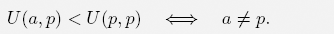
PROPOSITION 4.2. Assume that both information functions P1 and P2 are strict. Let E ⊆ be an arbitrary event. Assume that it is common knowledge for the players p1 and p1 in state σ* ∈ that they estimate the likelihood for E having occurred as η1 resp. η2. Then necessarily equality η1 = η2 holds.
Hence, if η1 ≠ η2, the players’ likelihood estimates cannot be common knowledge.
Proof. Consider the two events

Exactly in the event E1 ∩ E2, player p1 estimates the probability for the event E having occurred to be η1 while player p2’s estimate is η2.
Suppose E1 ∩ E2 is common knowledge in state σ*, i.e., there exists an event F ⊆ E1 ∩ E2 such that

Because the information function P1 is strict, F is the union of pairwise disjoint sets P1(σ1), . . . , P1(σk), say. Because of F ⊆ E1 ∩ E2, one has

Taking Ex. 4.14 into account, we therefore find

Similarly, Pr(E|F) = η2 is deduced and hence η2 = η1 follows.
EX. 4.14. Let A, B be events such that A ∩ B =  . Then the conditional probability satisfies:

______________________
1D. BERNOULLI (1700–1782).
2See, e.g., ROTANDO AND THORP [38].
3The notation differs in various parts of the world: in continental Europe, for example, the gross return rate r : 1 is customary.
4Mentioned to B. PASCAL (1623–1662).
5I have learned strategy (D) myself as a youth from my uncle Max.
6The normalized assumption results in no loss of generality: the analysis is independent of the size of B.
7See SHANNON [42].
8More can be found in, e.g., FAGIN et al. [10].