Chapter 5
Potentials, Utilities and Equilibria
Before discussing n-person games per se, it is useful to go back to the fundamental model of a game Γ being played on a system  of states and look at characteristic features of Γ. The aim is a general perspective on the numerical assessment of the value of states and strategic decisions.
1.Potentials and utilities
1.1.Potentials
To have a “potential” means to have the capability to enact something. In physics, the term potential refers to a characteristic quantity of a system whose change results in a dynamic behavior of the system. Potential energy, for example, may allow a mass to be set into motion. The resulting kinetic energy corresponds to the change in the potential. Gravity is thought to result from changes in a corresponding potential, the so-called gravitational field, and so on.
Mathematically, a potential is represented as a real-valued numerical parameter. In other words: A potential on the system  is a function

which assigns to a state σ ∈ a numerical value υ(σ). Of interest is the change in the potential resulting from a state transition σ → τ:

In fact, up to a constant, the potential υ : → ℝ is determined by its marginal potential ∂υ : × → ℝ:
LEMMA 5.1 For any potentials υ, w : → ℝ, the two statements are equivalent:
(1)∂υ = ∂w.
(2)There exists a constant K0 ∈ ℝ such that for all σ ∈ ,

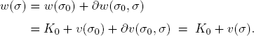
Proof. In the case (2), one has

and therefore (1). Conversely, if (1) holds, choose any σ0 and set K0 = w(σ0) – υ(σ0). Then for all σ ∈ , property (2) is apparent:

1.2.Utilities
A utility measure is a function

which we may interpret as a measuring device for the evaluation of a system transition σ → τ by a real number U(σ, τ). With U, we associate the so-called local utility functions ησ : → ℝ with the values

Hence the utility measure U can be equally well understood as an ensemble of local functions uσ : → ℝ:

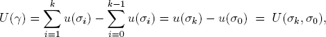
Path independence. Given the utility measure U, a path

of system transitions has the aggregated utility weight

We say that U is path independent if the utility weight of any path depends only on its initial state σ0 and the final state σk:

EX. 5.1. Show that U ∈ ℝ × is path independent if and only if the aggregated value of every circuit (i.e., path that starts and ends in the same state) is zero:

In particular, a path-independent U satisfies U(σ, σ) = 0.
Proof. If U is derived from the potential u : → ℝ, we have

and, therefore, for any γ = (σ0 → σ1 → . . . → σk−1 → σk):
which shows that U is path independent.
Conversely, assume that U is a path independent utility measure. Fix a state σ0 and consider the potential u ∈ ℝ with values

Since U is path independent, we have for all σ, τ ∈ ,

which implies

Utility potentials. We refer to υ ∈ ℝ as the underlying utility potential of a context that uses the marginal potential ∂υ as its utility measure. Such utility measures are particularly important in application models. The utility measures of cooperative game theory,1 for example, are typically derived from potentials.
2.Equilibria
When we talk about an “equilibrium” of an utility measure U ∈ ℝ× on the system , we make the prior assumption that each state σ has associated a neighborhood

and that we concentrate on state transitions to neighbors, i.e., to transitions of type σ → τ with τ ∈  σ.
σ.
We now say that a system state σ ∈ is a gain equilibrium of U if no feasible transition σ → τ to a neighbor state τ has a positive utility, i.e., if

Similarly, σ is a cost equilibrium if

REMARK 5.1 (Gains and costs). The negative C = −U of the utility measure U is also a utility measure and one finds:
σ is a gain equilibrium of U ⇔ σ is a cost equilibrium of C
From an abstract point of view, the theory of gain equilibria is equivalent to the theory of cost equilibria.
Many real-world systems appear to evolve in dynamic processes that eventually settle in an equilibrium state (or at least approximate an equilibrium) according to some utility measure. This phenomenon is strikingly observed in physics. But also economic theory has long suspected that economic systems may tend towards equilibrium states.2
2.1.Existence of equilibria
In practice, the determination of an equilibrium is typically a very difficult computational task. Moreover, many utilities do not even admit equilibria. It is generally not easy just to find out whether an equilibrium for a given utility exists at all. Therefore, one is interested in manageable conditions that allow one to conclude that at least one equilibrium exists.
Utilities from potentials. Consider a utility potential u : → ℝ with the marginal utility measure

Here, the following sufficient conditions offer themselves immediately:
(1) If  then σ is a gain equilibrium.
(2) If  then σ is a cost equilibrium.
Since every function on a finite set attains a maximum and a minimum, we find
PROPOSITION 5.2. If is finite, then every utility potential yields a utility measure with at least one gain and one cost equilibrium.
Similarly, we can derive the existence of equilibria in systems that are represented in a coordinate space.
Indeed, it is well-known that a continuous function on a compact set attains a maximum and a minimum.
REMARK 5.2. Notice that the conditions given in this section are sufficient to guarantee the existence of equilibria — no matter what neighborhood structure on is assumed.
Convex and concave utilities. If the utility measure U under consideration is not implied by a potential function, not even the finiteness of may be a guarantee for the existence of an equilibrium (see Ex. 5.2).
EX. 5.2. Give the example of a utility measure U relative to a finite state set with no gain and no cost equilibrium.
We now derive sufficient conditions for utilities U on a system whose set of states is represented by a nonempty convex set  ⊆ ℝm. We say:
•U is convex if every local function us : → ℝ is convex.
•U is concave if every local function us : → ℝ is concave.
THEOREM 5.1. Let U be a utility measure with continuous local utility functions us :  → ℝ on the nonempty compact set ⊆ ℝm. Then
(1)If U is convex, a cost equilibrium exists.
(2)If U is concave, a gain equilibrium exists.
Proof. Define the function G : × → ℝ with values

Then the hypothesis of the Theorem says that G satisfies the conditions of Corollary A.1 of the Appendix. Therefore, an element s ∈ exists such that

Consequently, s* is a gain equilibrium of U. (The convex case is proved in the same way.)
_____________________________
1 cf. Chapter 8.
2 A.A. COURNOT (1838–1877) [9].