
Diagonalization: Eigenvalues and Eigenvectors
9.1 Introduction
The ideas in this chapter can be discussed from two points of view.
Matrix Point of View
Suppose an n-square matrix A is given. The matrix A is said to be diagonalizable if there exists a nonsingular matrix P such that
is diagonal. This chapter discusses the diagonalization of a matrix A. In particular, an algorithm is given to find the matrix P when it exists.
Linear Operator Point of View
Suppose a linear operator T: V → V is given. The linear operator T is said to be diagonalizable if there exists a basis S of V such that the matrix representation of T relative to the basis S is a diagonal matrix D. This chapter discusses conditions under which the linear operator T is diagonalizable.
Equivalence of the Two Points of View
The above two concepts are essentially the same. Specifically, a square matrix A may be viewed as a linear operator F defined by

where X is a column vector, and B = P−1 AP represents F relative to a new coordinate system (basis) S whose elements are the columns of P. On the other hand, any linear operator T can be represented by a matrix A relative to one basis and, when a second basis is chosen, T is represented by the matrix
where P is the change-of-basis matrix.
Most theorems will be stated in two ways: one in terms of matrices A and again in terms of linear mappings T.
Role of Underlying Field K
The underlying number field K did not play any special role in our previous discussions on vector spaces and linear mappings. However, the diagonalization of a matrix A or a linear operator T will depend on the roots of a polynomial Δ(t) over K, and these roots do depend on K. For example, suppose Δ(t) = t2 + 1. Then Δ(t) has no roots if K = R, the real field; but Δ(t) has roots ±i if K = C, the complex field. Furthermore, finding the roots of a polynomial with degree greater than two is a subject unto itself (frequently discussed in numerical analysis courses). Accordingly, our examples will usually lead to those polynomials Δ(t) whose roots can be easily determined.
9.2 Polynomials of Matrices
Consider a polynomial f(t) = antn + · · · + a1t + a0 over a field K. Recall (Section 2.8) that if A is any square matrix, then we define

I where I is the identity matrix. In particular, we say that A is a root of f(t) if f(A) = 0, the zero matrix.
 . Then
 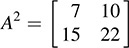 . Let
. Let
Then

and

Thus, A is a zero of g(t).
The following theorem (proved in Problem 9.7) applies.
THEOREM 9.1: Let f and g be polynomials. For any square matrix A and scalar k,
(i) (f + g)(A) = f (A) + g(A)
(ii) (fg)(A) = f (A)g(A)
(iii) (kf)(A) = kf (A)
(iv) f (A)g(A) = g(A) f (A).
Observe that (iv) tells us that any two polynomials in A commute.
Matrices and Linear Operators
Now suppose that T: V → V is a linear operator on a vector space V. Powers of T are defined by the composition operation:

Also, for any polynomial f (t) = antn + · · · + a1t + a0, we define f (T) in the same way as we did for matrices:

where I is now the identity mapping. We also say that T is a zero or root of f (t) if f (T) = 0, the zero mapping. We note that the relations in Theorem 9.1 hold for linear operators as they do for matrices.
Remark: Suppose A is a matrix representation of a linear operator T. Then f(A) is the matrix representation of f(T), and, in particular, f(T) = 0 if and only if f(A) = 0.
9.3 Characteristic Polynomial, Cayley–Hamilton Theorem
Let A = [aij] be an n-square matrix. The matrix M = A tIn, where In is the n-square identity matrix and t is an indeterminate, may be obtained by subtracting t down the diagonal of A. The negative of M is the matrix tIn − A, and its determinant

which is a polynomial in t of degree n and is called the characteristic polynomial of A.
We state an important theorem in linear algebra (proved in Problem 9.8).
THEOREM 9.2: (Cayley–Hamilton) Every matrix A is a root of its characteristic polynomial.
Remark: Suppose A =[aij] is a triangular matrix. Then tI − A is a triangular matrix with diagonal entries t − aii; hence,

Observe that the roots of Δ(t) are the diagonal elements of A.
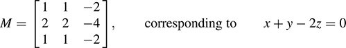
EXAMPLE 9.2 Let  . Its characteristic polynomial is

As expected from the Cayley–Hamilton theorem, A is a root of Δ(t); that is,

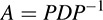
Now suppose A and B are similar matrices, say B = P−1AP, where P is invertible. We show that A and B have the same characteristic polynomial. Using tI = P−1tIP, we have
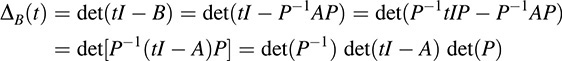
Using the fact that determinants are scalars and commute and that det(P−1 det(P) = 1, we finally obtain

Thus, we have proved the following theorem.
THEOREM 9.3: Similar matrices have the same characteristic polynomial.
Characteristic Polynomials of Degrees 2 and 3
There are simple formulas for the characteristic polynomials of matrices of orders 2 and 3.
(a) Suppose  . Then

Here tr(A) denotes the trace of A—that is, the sum of the diagonal elements of A.
(b) Suppose  . Then

(Here A11, A22, A33 denote, respectively, the cofactors of a11, a22, a33.)
EXAMPLE 9.3 Find the characteristic polynomial of each of the following matrices:


(a) We have tr(A) = 5 + 10 = 15 and |A| = 50 − 6 = 44; hence, Δ(t) + t2 − 15t + 44.
(b) We have tr(B) = 7 + 2 = 9 and |B| = 14 + 6 = 20; hence, Δ(t) = t2 − 9t + 20.
(c) We have tr(C) = 5 − 4 = 1 and |C| = 20 + 8 = 12; hence, Δ(t) = t2 − t − 12.
EXAMPLE 9.4 Find the characteristic polynomial of  .
.
We have tr(A) = 1 + 3 + 9 = 13. The cofactors of the diagonal elements are as follows:

Thus, A11 + A22 + A33 = 31. Also, |A| = 27 + 2 + 0 − 6 − 6 − 0 = 17. Accordingly,

Remark: The coefficients of the characteristic polynomial Δ(t) of the 3-square matrix A are, with alternating signs, as follows:

We note that each Sk is the sum of all principal minors of A of order k.
The next theorem, whose proof lies beyond the scope of this text, tells us that this result is true in general.
THEOREM 9.4: Let A be an n-square matrix. Then its characteristic polynomial is

where Sk is the sum of the principal minors of order k.
Characteristic Polynomial of a Linear Operator
Now suppose T: V → V is a linear operator on a vector space V of finite dimension. We define the characteristic polynomial Δ(t) of T to be the characteristic polynomial of any matrix representation of T. Recall that if A and B are matrix representations of T, then B = P−1AP, where P is a change-of-basis matrix. Thus, A and B are similar, and by Theorem 9.3, A and B have the same characteristic polynomial. Accordingly, the characteristic polynomial of T is independent of the particular basis in which the matrix representation of T is computed.
Because f(T) = 0 if and only if f(A) = 0, where f(t) is any polynomial and A is any matrix representation of T, we have the following analogous theorem for linear operators.
THEOREM 9.2′: (Cayley–Hamilton) A linear operator T is a zero of its characteristic polynomial.
9.4 Diagonalization, Eigenvalues and Eigenvectors
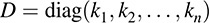
Let A be any n-square matrix. Then A can be represented by (or is similar to) a diagonal matrix D = diag(k1, k2, …, kn) if and only if there exists a basis S consisting of (column) vectors u1, u2, …, un such that

In such a case, A is said to be diagonizable. Furthermore, D = P−1 AP, where P is the nonsingular matrix whose columns are, respectively, the basis vectors u1, u2, …, un.
The above observation leads us to the following definition.
DEFINITION: Let A be any square matrix. A scalar λ is called an eigenvalue of A if there exists a nonzero (column) vector υ such that

Any vector satisfying this relation is called an eigenvector of A belonging to the eigenvalueλ.
We note that each scalar multiple kυ of an eigenvector υ belonging to λ is also such an eigenvector, because

The set Eλ of all such eigenvectors is a subspace of V (Problem 9.19), called the eigenspace of λ. (If dim Eλ = 1, then Eλ is called an eigenline and λ is called a scaling factor.)
The terms characteristic value and characteristic vector (or proper value and proper vector) are sometimes used instead of eigenvalue and eigenvector.
The above observation and definitions give us the following theorem.
THEOREM 9.5: An n-square matrix A is similar to a diagonal matrix D if and only if A has n linearly independent eigenvectors. In this case, the diagonal elements of D are the corresponding eigenvalues and D = P−1AP, where P is the matrix whose columns are the eigenvectors.
Suppose a matrix A can be diagonalized as above, say P−1 AP = D, where D is diagonal. Then A has the extremely useful diagonal factorization:
Using this factorization, the algebra of A reduces to the algebra of the diagonal matrix D, which can be easily calculated. Specifically, suppose D = diag(k1, k2, …, kn). Then

More generally, for any polynomial f(t),

Furthermore, if the diagonal entries of D are nonnegative, let

Then B is a nonnegative square root of A; that is, B2 = A and the eigenvalues of B are nonnegative.
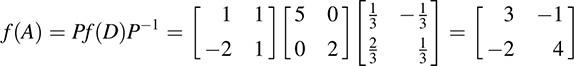
EXAMPLE 9.5 Let  and
and  and
and  . Then

Thus, υ1 and υ2 are eigenvectors of A belonging, respectively, to the eigenvalues λ1 = 1 and λ2 = 4. Observe that υ1 and υ2 are linearly independent and hence form a basis of R2. Accordingly, A is diagonalizable. Furthermore, let P be the matrix whose columns are the eigenvectors υ1 and υ2. That is, let
Then A is similar to the diagonal matrix

As expected, the diagonal elements 1 and 4 in D are the eigenvalues corresponding, respectively, to the eigenvectors υ1 and υ2, which are the columns of P. In particular, A has the factorization

Accordingly,
Moreover, suppose f(t) = t3 − 5t2 + 3t + 6; hence, f (1) = 5 and f (4) = 2. Then
Last, we obtain a “positive square root” of A. Specifically, using  and
and  , we obtain the matrix
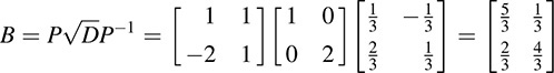
where B2 = A and where B has positive eigenvalues 1 and 2.
Remark: Throughout this chapter, we use the following fact:

That is, P−1 is obtained by interchanging the diagonal elements a and d of P, taking the negatives of the nondiagonal elements b and c, and dividing each element by the determinant |P|.
Properties of Eigenvalues and Eigenvectors
Example 9.5 indicates the advantages of a diagonal representation (factorization) of a square matrix. In the following theorem (proved in Problem 9.20), we list properties that help us to find such a representation.
THEOREM 9.6: Let A be a square matrix. Then the following are equivalent.
(i) A scalar λ is an eigenvalue of A.
(ii) The matrix M = A − λI is singular.
(iii) The scalar λ is a root of the characteristic polynomial Δ(t) of A.
The eigenspace Eλ of an eigenvalue λ is the solution space of the homogeneous system MX = 0, where M = A λI; that is, M is obtained by subtracting λ down the diagonal of A.
Some matrices have no eigenvalues and hence no eigenvectors. However, using Theorem 9.6 and the Fundamental Theorem of Algebra (every polynomial over the complex field C has a root), we obtain the following result.
THEOREM 9.7: Let A be a square matrix over the complex field C. Then A has at least one eigenvalue.
The following theorems will be used subsequently. (The theorem equivalent to Theorem 9.8 for linear operators is proved in Problem 9.21, and Theorem 9.9 is proved in Problem 9.22.)
THEOREM 9.8: Suppose υ1, υ2, …, υn are nonzero eigenvectors of a matrix A belonging to distinct eigenvalues λ1, λ2, …, λn. Then υ1, υ2, …, υn are linearly independent.
THEOREM 9.9: Suppose the characteristic polynomial Δ(t) of an n-square matrix A is a product of n distinct factors, say, Δ(t) = (t − a1)(t − a2)(t − an). Then A is similar to the diagonal matrix D = diag(a1, a2, …, an).
If λ is an eigenvalue of a matrix A, then the algebraic multiplicity of λ is defined to be the multiplicity of λ as a root of the characteristic polynomial of A, and the geometric multiplicity of λ is defined to be the dimension of its eigenspace, dim Eλ. The following theorem (whose equivalent for linear operators is proved in Problem 9.23) holds.
THEOREM 9.10: The geometric multiplicity of an eigenvalue λ of a matrix A does not exceed its algebraic multiplicity.
Diagonalization of Linear Operators
Consider a linear operator T: V → V. Then T is said to be diagonalizable if it can be represented by a diagonal matrix D. Thus, T is diagonalizable if and only if there exists a basis S = {u1, u2, …, un} of V for which

In such a case, T is represented by the diagonal matrix
relative to the basis S.
The above observation leads us to the following definitions and theorems, which are analogous to the definitions and theorems for matrices discussed above.
DEFINITION: Let T be a linear operator. A scalar λ is called an eigenvalue of T if there exists a nonzero vector υ such that T(υ) = λ υ. Every vector satisfying this relation is called an eigenvector of T belonging to the eigenvalue λ.
The set Eλ of all eigenvectors belonging to an eigenvalue λ is a subspace of V, called the eigenspace of λ. (Alternatively, λ is an eigenvalue of T if λI − T is singular, and, in this case, Eλ is the kernel of λI − T.) The algebraic and geometric multiplicities of an eigenvalue λ of a linear operator T are defined in the same way as those of an eigenvalue of a matrix A.
The following theorems apply to a linear operator T on a vector space V of finite dimension.
THEOREM 9.5′: T can be represented by a diagonal matrix D if and only if there exists a basis S of V consisting of eigenvectors of T. In this case, the diagonal elements of D are the corresponding eigenvalues.
THEOREM 9.6′: Let T be a linear operator. Then the following are equivalent:
(i) A scalar λ is an eigenvalue of T.
(ii) The linear operator λI − T is singular.
(iii) The scalar λ is a root of the characteristic polynomial Δ(t) of T.
THEOREM 9.7′: Suppose V is a complex vector space. Then T has at least one eigenvalue.
THEOREM 9.8′: Suppose υ1, υ2, …, υn are nonzero eigenvectors of a linear operator T belonging to distinct eigenvalues λ1, λ2, …, λn. Then υ1, υ2, …, υn are linearly independent.
THEOREM 9.9′: Suppose the characteristic polynomial Δ(t) of T is a product of n distinct factors, say, Δ(t) = (t − a1)(t − a2) · · · (t − an). Then T can be represented by the diagonal matrix D = diag(a1, a2, …, an).
THEOREM 9.10′: The geometric multiplicity of an eigenvalue λ of T does not exceed its algebraic multiplicity.
Remark: The following theorem reduces the investigation of the diagonalization of a linear operator T to the diagonalization of a matrix A.
THEOREM 9.11: Suppose A is a matrix representation of T. Then T is diagonalizable if and only if A is diagonalizable.
9.5 Computing Eigenvalues and Eigenvectors, Diagonalizing Matrices
This section gives an algorithm for computing eigenvalues and eigenvectors for a given square matrix A and for determining whether or not a nonsingular matrix P exists such that P−1 AP is diagonal.
ALGORITHM 9.1: (Diagonalization Algorithm) The input is an n-square matrix A.
Step 1. Find the characteristic polynomial Δ(t) of A.
Step 2. Find the roots of Δ(t) to obtain the eigenvalues of A.
Step 3. Repeat (a) and (b) for each eigenvalue λ of A.
(a) Form the matrix M = A − λI by subtracting λ down the diagonal of A.
(b) Find a basis for the solution space of the homogeneous system MX = 0. (These basis vectors are linearly independent eigenvectors of A belonging to λ.)
Step 4. Consider the collection S = {υ1, υ2, …, υm} of all eigenvectors obtained in Step 3.
(a) If m ≠ n, then A is not diagonalizable.
(b) If m = n, then A is diagonalizable. Specifically, let P be the matrix whose columns are the eigenvectors υ1, υ2, …, υn. Then

where λi is the eigenvalue corresponding to the eigenvector υi.
EXAMPLE 9.6 The diagonalization algorithm is applied to  ,
,
(1) The characteristic polynomial Δ(t) of A is computed:

(2) Set Δ(t) = t2 − 3t − 10 = (t − 5)(t + 2) = 0. The roots λ1 = 5 and λ2 = 2 are the eigenvalues of A.
(3) (i) We find an eigenvector v1 of A belonging to the eigenvalue λ1 = 5. Subtract λ1 = 5 down the diagonal of A to obtain the matrix

The system has only one independent solution, for example, v1 = (2, 1).
(ii) We find an eigenvector v2 of A belonging to the eigenvalue λ2 = −2. Subtract −2 (or add 2) down the diagonal of A to obtain the matrix

The system has only one independent solution, for example, v2 = (−1, 3).
(4) Let P be the matrix whose columns are the eigenvectors v1 and v2. Then  . Thus D = P−1AP is the diagonal matrix whose diagonal entries are the corresponding eigenvalues:

Remark: Find a 2 × 2 matrix A with eigenvalues λ1 = 2 and λ2 = 3 and corresponding eigenvectors v1 = (1, 3) and v2 = (1, 4). We know that P−1AP = D where  and
and  .
.

EXAMPLE 9.7 Consider the matrix  . We have

Accordingly, λ = 4 is the only eigenvalue of B.
Subtract λ = 4 down the diagonal of B to obtain the matrix

The system has only one independent solution; for example, x = 1, y = 1. Thus, υ = (1, 1) and its multiples are the only eigenvectors of B. Accordingly, B is not diagonalizable, because there does not exist a basis consisting of eigenvectors of B.
EXAMPLE 9.8 Consider the matrix  . Here tr(A) = 3 − 3 = 0 and |A| = 9 + 10 = 1. Thus, Δ(t) = t2 + 1 is the characteristic polynomial of A. We consider two cases:
(a) A is a matrix over the real field R. Then Δ(t) has no (real) roots. Thus, A has no eigenvalues and no eigenvectors, and so A is not diagonalizable.
(b) A is a matrix over the complex field C. Then Δ(t) = (t − i)(t + i) has two roots, i and −i. Thus, A has two distinct eigenvalues i and −i, and hence, A has two independent eigenvectors. Accordingly there exists a nonsingular matrix P over the complex field C for which
Therefore, A is diagonalizable (over C).
9.6 Diagonalizing Real Symmetric Matrices and Quadratic Forms
There are many real matrices A that are not diagonalizable. In fact, some real matrices may not have any (real) eigenvalues. However, if A is a real symmetric matrix, then these problems do not exist. Namely, we have the following theorems.
THEOREM 9.12: Let A be a real symmetric matrix. Then each root λ of its characteristic polynomial is real.
THEOREM 9.13: Let A be a real symmetric matrix. Suppose u and υ are eigenvectors of A belonging to distinct eigenvalues λ1 and λ2. Then u and υ are orthogonal, that; is, 〈u〉, υ = 0.
The above two theorems give us the following fundamental result.
THEOREM 9.14: Let A be a real symmetric matrix. Then there exists an orthogonal matrix P such that D = P−1AP is diagonal.
The orthogonal matrix P is obtained by normalizing a basis of orthogonal eigenvectors of A as illustrated below. In such a case, we say that A is“orthogonally diagonalizable.”
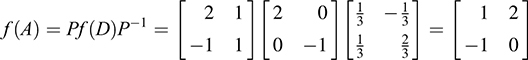
EXAMPLE 9.9 Let  , a real symmetric matrix. Find an orthogonal matrix P such that P−1AP is diagonal.
First we find the characteristic polynomial Δ(t) of A. We have

Accordingly, λ1 = 6 and λ2 = 1 are the eigenvalues of A.
(a) Subtracting λ1 = 6 down the diagonal of A yields the matrix

A nonzero solution is u1 = (1, −2).
(b) Subtracting λ2 = 1 down the diagonal of A yields the matrix

(The second equation drops out, because it is a multiple of the first equation.) A nonzero solution is u2 = (2, 1).
As expected from Theorem 9.13, u1 and u2 are orthogonal. Normalizing u1 and u2 yields the orthonormal vectors

Finally, let P be the matrix whose columns are  and
and  , respectively. Then

As expected, the diagonal entries of P−1AP are the eigenvalues corresponding to the columns of P.
The procedure in the above Example 9.9 is formalized in the following algorithm, which finds an orthogonal matrix P such that P−1AP is diagonal.
ALGORITHM 9.2: (Orthogonal Diagonalization Algorithm) The input is a real symmetric matrix A.
Step 1. Find the characteristic polynomial Δ(t) of A.
Step 2. Find the eigenvalues of A, which are the roots of Δ(t).
Step 3. For each eigenvalue λ of A in Step 2, find an orthogonal basis of its eigenspace.
Step 4. Normalize all eigenvectors in Step 3, which then forms an orthonormal basis of Rn.
Step 5. Let P be the matrix whose columns are the normalized eigenvectors in Step 4.
Application to Quadratic Forms
Let q be a real polynomial in variables x1, x2, …, xn such that every term in q has degree two; that is,

Then q is called a quadratic form. If there are no cross-product terms xixj (i.e., all dij = 0), then q is said to be diagonal.
The above quadratic form q determines a real symmetric matrix A = [aij], where aii = ci and  . Namely, q can be written in the matrix form

where X = [x1, x2, …, xn]T is the column vector of the variables. Furthermore, suppose X = PY is a linear substitution of the variables. Then substitution in the quadratic form yields

Thus, PTAP is the matrix representation of q in the new variables.
We seek an orthogonal matrix P such that the orthogonal substitution X = PY yields a diagonal quadratic form for which PTAP is diagonal. Because P is orthogonal, PT = P−1, and hence, PTAP = P−1AP. The above theory yields such an orthogonal matrix P.
EXAMPLE 9.10 Consider the quadratic form

By Example 9.9,

Let Y = [s, t]T: Then matrix P corresponds to the following linear orthogonal substitution x = PY of the variables x and y in terms of the variables s and t:

This substitution in q(x, y) yields the diagonal quadratic form q(s, t) = 6s2 + t2.
9.7 Minimal Polynomial
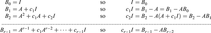
Let A be any square matrix. Let J(A) denote the collection of all polynomials f(t) for which A is a root—that is, for which f(A) = 0. The set J(A) is not empty, because the Cayley–Hamilton Theorem 9.1 tells us that the characteristic polynomial ΔA(t) of A belongs to J(A). Let m(t) denote the monic polynomial of lowest degree in J(A). (Such a polynomial m(t) exists and is unique.) We call m(t) the minimal polynomial of the matrix A.
Remark: A polynomial f(t) ≠ 0 is monic if its leading coefficient equals one.
The following theorem (proved in Problem 9.33) holds.
THEOREM 9.15: The minimal polynomial m(t) of a matrix (linear operator) A divides every polynomial that has A as a zero. In particular, m(t) divides the characteristic polynomial Δ(t) of A.
There is an even stronger relationship between m(t) and Δ(t).
THEOREM 9.16: The characteristic polynomial Δ(t) and the minimal polynomial m(t) of a matrix A have the same irreducible factors.
This theorem (proved in Problem 9.35) does not say that m(t) = Δ(t), only that any irreducible factor of one must divide the other. In particular, because a linear factor is irreducible, m(t) and Δ(t) have the same linear factors. Hence, they have the same roots. Thus, we have the following theorem.
THEOREM 9.17: A scalar λ is an eigenvalue of the matrix A if and only if λ is a root of the minimal polynomial of A.
EXAMPLE 9.11 Find the minimal polynomial m(t) of  .
.
First find the characteristic polynomial Δ(t) of A. We have

Hence,

The minimal polynomial m(t) must divide Δ(t). Also, each irreducible factor of Δ(t) (i.e., t − 1 and t − 3) must also be a factor of m(t). Thus, m(t) is exactly one of the following:

We know, by the Cayley–Hamilton theorem, that g(A) = Δ(A) = 0. Hence, we need only test f(t). We have

Thus, f(t) = m(t) = (t − 1)(t − 3) = t2 − 4t + 3 is the minimal polynomial of A.
(a) Consider the following two r-square matrices, where a ≠ 0:

The first matrix, called a Jordan Block, has λ’s on the diagonal, 1’s on the superdiagonal (consisting of the entries above the diagonal entries), and 0’s elsewhere. The second matrix A has λ’s on the diagonal, a’s on the superdiagonal, and 0’s elsewhere. [Thus, A is a generalization of J(λ, r).] One can show that

is both the characteristic and minimal polynomial of both J(λ, r) and A.
(b) Consider an arbitrary monic polynomial:

Let C(f) be the n-square matrix with 1’s on the subdiagonal (consisting of the entries below the diagonal entries), the negatives of the coefficients in the last column, and 0’s elsewhere as follows:

Then C(f) is called the companion matrix of the polynomial f(t). Moreover, the minimal polynomial m(t) and the characteristic polynomial Δ(t) of the companion matrix C(f) are both equal to the original polynomial f(t).
Minimal Polynomial of a Linear Operator
The minimal polynomial m(t) of a linear operator T is defined to be the monic polynomial of lowest degree for which T is a root. However, for any polynomial f(t), we have

where A is any matrix representation of T. Accordingly, T and A have the same minimal polynomials. Thus, the above theorems on the minimal polynomial of a matrix also hold for the minimal polynomial of a linear operator. That is, we have the following theorems.
THEOREM 9.15′: The minimal polynomial m(t) of a linear operator T divides every polynomial that has T as a root. In particular, m(t) divides the characteristic polynomial Δ(t) of T.
THEOREM 9.16′: The characteristic and minimal polynomials of a linear operator T have the same irreducible factors.
THEOREM 9.17′: A scalar λ is an eigenvalue of a linear operator T if and only if λ is a root of the minimal polynomial m(t) of T.
9.8 Characteristic and Minimal Polynomials of Block Matrices
This section discusses the relationship of the characteristic polynomial and the minimal polynomial to certain (square) block matrices.
Characteristic Polynomial and Block Triangular Matrices
Suppose M is a block triangular matrix, say  , where A1 and A2 are square matrices. Then tI − M is also a block triangular matrix, with diagonal blocks tI − A1 and tI − A2. Thus,

That is, the characteristic polynomial of M is the product of the characteristic polynomials of the diagonal blocks A1 and A2.
By induction, we obtain the following useful result.
THEOREM 9.18: Suppose M is a block triangular matrix with diagonal blocks A1, A2, …, Ar. Then the characteristic polynomial of M is the product of the characteristic polynomials of the diagonal blocks Ai; that is,

EXAMPLE 9.13 Consider the matrix  .
.
Then M is a block triangular matrix with diagonal blocks 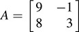 and
and  . Here

Accordingly, the characteristic polynomial of M is the product

Minimal Polynomial and Block Diagonal Matrices
The following theorem (proved in Problem 9.36) holds.
THEOREM 9.19: Suppose M is a block diagonal matrix with diagonal blocks A1, A2, …, Ar. Then the minimal polynomial of M is equal to the least common multiple (LCM) of the minimal polynomials of the diagonal blocks Ai.
Remark: We emphasize that this theorem applies to block diagonal matrices, whereas the analogous Theorem 9.18 on characteristic polynomials applies to block triangular matrices.
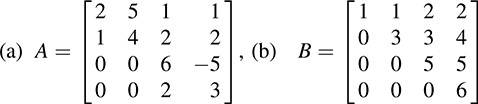
EXAMPLE 9.14 Find the characteristic polynomal Δ(t) and the minimal polynomial m(t) of the block diagonal matrix:

Then Δ(t) is the product of the characterization polynomials Δ1(t), Δ2(t), Δ3(t) of A1, A2, A3, respectively. One can show that

Thus, Δ(t) = (t − 2)3(t − 7)2. [As expected, deg Δ(t) = 5.]
The minimal polynomials m1(t), m2(t), m3(t) of the diagonal blocks A1, A2, A3, respectively, are equal to the characteristic polynomials; that is,

But m(t) is equal to the least common multiple of m1(t), m2(t), m3(t). Thus, m(t) = (t − 2)2(t − 7).
SOLVED PROBLEMS
Polynomials of Matrices, Characteristic Polynomials
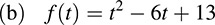
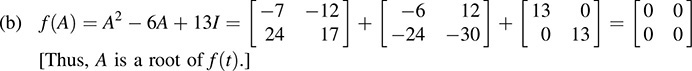
 . Find f(A), where
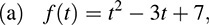


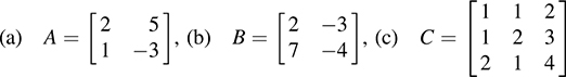
9.2. Find the characteristic polynomial Δ(t) of each of the following matrices:


Use the formula (t) = t2 − tr(M) t + |M| for a 2 × 2 matrix M:
(a) tr(A) = 2 + 1 = 3, |A| = 2 − 20 = −18, so Δ(t) = t2 − 3t − 18
(b) tr(B) = 7 − 2 = 5, |B| = 14 + 15 = 1, so Δ(t) = t2 − 5t + 1
(c) tr(C) = 3 − 3 = 0, |C| = 9 + 18 = 9, so Δ(t) = t + 2 + 9
9.3. Find the characteristic polynomial Δ(t) of each of the following matrices:

Use the formula Δ(t) = t3 − tr(A)t2 + (A11 + A22 + A33)t − |A|, where Aii is the cofactor of aii in the 3 − 3 matrix A = [aij].
(a) tr(A) = 1 + 0 + 5 = 6,

Thus,

(b) tr(B) = 1 + 2 − 4 = −1

Thus,

9.4. Find the characteristic polynomial Δ(t) of each of the following matrices:
(a) A is block triangular with diagonal blocks


(b) Because B is triangular, Δ(t) = (t − 1)(t − 3)(t − 5)(t − 6).
9.5. Find the characteristic polynomial Δ(t) of each of the following linear operators:
(a) F: R2 → R2 defined by F(x, y) = (3x + 5y; 2x − 7y).
(b) D: V → V defined by D(f) = df/dt, where V is the space of functions with basis S = {sin t, cos t}.
The characteristic polynomial Δ(t) of a linear operator is equal to the characteristic polynomial of any matrix A that represents the linear operator.
(a) Find the matrix A that represents T relative to the usual basis of R2. We have

(b) Find the matrix A representing the differential operator D relative to the basis S. We have


9.6. Show that a matrix A and its transpose AT have the same characteristic polynomial.
By the transpose operation, (tI − A)T = tIT − AT = tI − AT. Because a matrix and its transpose have the same determinant,

9.7. Prove Theorem 9.1: Let f and g be polynomials. For any square matrix A and scalar k,
(i) (f + g)(A) = f(A) + g(A),
(ii) (fg)(A) = f(A)g(A),
(iii) (kf)(A) = kf(A),
(iv) f(A)g(A) = g(A)f(A).
Suppose f = antn + · · · + a1t + a0 and g = bmtm + · · · + b1t + b0. Then, by definition,

(i) Suppose m ≤ n and let bi = 0 if i > m. Then

Hence,

(ii) By definition,  , where

Hence, 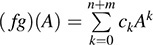 and
and

(iii) By definition, kf = kantn · · · + ka1t + ka0, and so

(iv) By (ii), g(A)f(A) = (gf)(A) = (fg)(A) = f(A)g(A).
9.8. Prove the Cayley–Hamilton Theorem 9.2: Every matrix A is a root of its characterstic polynomial Δ(t).
Let A be an arbitrary n-square matrix and let Δ(t) be its characteristic polynomial, say,

Now let B(t) denote the classical adjoint of the matrix tI − A. The elements of B(t) are cofactors of the matrix tI − A and hence are polynomials in t of degree not exceeding n − 1. Thus,

where the Bi are n-square matrices over K which are independent of t. By the fundamental property of the classical adjoint (Theorem 8.9), (tI − A)B(t) = |tI − A|I, or

Removing the parentheses and equating corresponding powers of t yields

Multiplying the above equations by An, An − 1, …, A, I, respectively, yields

Adding the above matrix equations yields 0 on the left-hand side and Δ(A) on the right-hand side; that is,

Therefore, Δ(A) = 0, which is the Cayley–Hamilton theorem.
Eigenvalues and Eigenvectors of 2 × 2 Matrices
 .
.(a) Find all eigenvalues and corresponding eigenvectors.
(b) Find matrices P and D such that P is nonsingular and D = P−1AP is diagonal.
(a) First find the characteristic polynomial Δ(t) of A:

The roots λ = 2 and λ = 5 of Δ(t) are the eigenvalues of A. We find corresponding eigenvectors.
(i) Subtract λ = 2 down the diagonal of A to obtain the matrix M = A − 2I, where the corresponding homogeneous system MX = 0 yields the eigenvectors corresponding to λ = 2. We have

The system has only one free variable, and υ1 = (4, 1) is a nonzero solution. Thus, υ1 = (4, 1) is an eigenvector belonging to (and spanning the eigenspace of) λ = 2.
(ii) Subtract λ = −5 (or, equivalently, add 5) down the diagonal of A to obtain

The system has only one free variable, and υ2 = (1, 2) is a nonzero solution. Thus, υ2 = (1, 2) is an eigenvector belonging to λ = 5.
(b) Let P be the matrix whose columns are υ1 and υ2. Then

Note that D is the diagonal matrix whose diagonal entries are the eigenvalues of A corresponding to the eigenvectors appearing in P.
Remark: Here P is the change-of-basis matrix from the usual basis of R2 to the basis S = {υ1, υ2}, and D is the matrix that represents (the matrix function) A relative to the new basis S.
 .
.(a) Find all eigenvalues and corresponding eigenvectors.
(b) Find a nonsingular matrix P such that D = P−1AP is diagonal, and P−1.
(c) Find A6 and f(A), where t4 − 3t3 − 6t2 + 7t + 3.
(d) Find a “real cube root” of B—that is, a matrix B such that B3 = A and B has real eigenvalues.
(a) First find the characteristic polynomial Δ(t) of A:

The roots λ = 1 and λ = 4 of Δ(t) are the eigenvalues of A. We find corresponding eigenvectors.
(i) Subtract λ = 1 down the diagonal of A to obtain the matrix M = A − λI, where the corresponding homogeneous system MX = 0 yields the eigenvectors belonging to λ = 1. We have

The system has only one independent solution; for example, x = 2, y = 1. Thus, υ1 = (2, −1) is an eigenvector belonging to (and spanning the eigenspace of) λ = 1.
(ii) Subtract λ = 4 down the diagonal of A to obtain

The system has only one independent solution; for example, x = 1, y = 1. Thus, υ2 = (1, 1) is an eigenvector belonging to λ = 4.
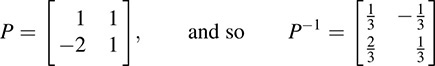
(b) Let P be the matrix whose columns are υ1 and υ2. Then

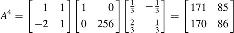
(c) Using the diagonal factorization A = PDP−1, and 16 = 1 and 46 = 4096, we get

Also, f (1) = 2 and f (4) = 1. Hence,
(d) Here  is the real cube root of D. Hence the real cube root of A is

9.11. Each of the following real matrices defines a linear transformation on R2:

Find, for each matrix, all eigenvalues and a maximum set S of linearly independent eigenvectors. Which of these linear operators are diagonalizable—that is, which can be represented by a diagonal matrix?
(a) First find Δ(t) = t2 − 3t − 28 = (t − 7)(t + 4). The roots λ = 7 and λ = 4 are the eigenvalues of A. We find corresponding eigenvectors.
(i) Subtract λ = 7 down the diagonal of A to obtain

Here υ1 = (3, 1) is a nonzero solution.
(ii) Subtract λ = −4 (or add 4) down the diagonal of A to obtain

Here υ2 = (2, −3) is a nonzero solution.
Then S = {υ1, υ2} = {(3, 1), (2, −3)} is a maximal set of linearly independent eigenvectors. Because S is abasisof R2, A is diagonalizable. Using the basis S, A is represented by the diagonal matrix D = diag(7, −4).
(b) First find the characteristic polynomial Δ(t) = t2 + 1. There are no real roots. Thus B, a real matrix representing a linear transformation on R2, has no eigenvalues and no eigenvectors. Hence, in particular, B is not diagonalizable.
(c) First find Δ(t) = t2 − 8t + 16 = (t − 4)2. Thus, λ = 4 is the only eigenvalue of C. Subtract λ = 4 down the diagonal of C to obtain

The homogeneous system has only one independent solution; for example, x = 1, y = 1. Thus, υ = (1, 1) is an eigenvector of C. Furthermore, as there are no other eigenvalues, the singleton set S = {υ} = {(1, 1)} is a maximal set of linearly independent eigenvectors of C. Furthermore, because S is not a basis of R2, C is not diagonalizable.
9.12. Suppose the matrix B in Problem 9.11 represents a linear operator on complex space C2. Show that, in this case, B is diagonalizable by finding a basis S of C2 consisting of eigenvectors of B.
The characteristic polynomial of B is still Δ(t) = t2 + 1. As a polynomial over C, Δ(t) does factor; specifically, Δ(t) = (t − i)(t + i). Thus, λ = i and λ = i are the eigenvalues of B.
(i) Subtract λ = i down the diagonal of B to obtain the homogeneous system

The system has only one independent solution; for example, x = 1, y = 1 − i. Thus, υ1 = (1, 1 − i) is an eigenvector that spans the eigenspace of λ = i.
(ii) Subtract λ = i (or add i) down the diagonal of B to obtain the homogeneous system

The system has only one independent solution; for example, x = 1, y = 1 + i. Thus, υ2 = (1, 1 + i) is an eigenvector that spans the eigenspace of λ = i.
As a complex matrix, B is diagonalizable. Specifically, S = {υ1, υ2} = {(1, 1 − i), (1, 1 + i)} is a basis of C2 consisting of eigenvectors of B. Using this basis S, B is represented by the diagonal matrix D = diag(i, −i).
9.13. Let L be the linear transformation on R2 that reflects each point P across the line y = kx, where k > 0. (See Fig. 9-1.)
(a) Show that υ1 = (k, 1) and υ2 = (1, −k) are eigenvectors of L.
(b) Show that L is diagonalizable, and find a diagonal representation D.

(a) The vector υ1 = (k, 1) lies on the line y = kx, and hence is left fixed by L; that is, L(υ1) = υ1. Thus, υ1 is an eigenvector of L belonging to the eigenvalue λ1 = 1.
The vector υ2 = (1, − k) is perpendicular to the line y = kx, and hence, L reflects υ2 into its negative; that is, L(υ2) = υ2. Thus, υ2 is an eigenvector of L belonging to the eigenvalue λ2 = 1.
(b) Here S = {υ1, υ2} is a basis of R2 consisting of eigenvectors of L. Thus, L is diagonalizable, with the diagonal representation 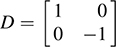 (relative to the basis S).
Eigenvalues and Eigenvectors
9.14. Let  . (a) Find all eigenvalues of A.
(b) Find a maximum set S of linearly independent eigenvectors of A.
(c) Is A diagonalizable? If yes, find P such that D = P−1AP is diagonal.
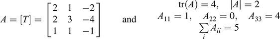
(a) First find the characteristic polynomial Δ(t) of A. We have

Also, find each cofactor Aii of aii in A:

Hence,

Assuming Δt has a rational root, it must be among ±1, ±3, ±5, ±9, ±15, ±45. Testing, by synthetic division, we get

Thus, t = 3 is a root of Δ(t). Also, t − 3 is a factor and t2 − 8t + 15 is a factor. Hence,

Accordingly, λ = 3 and λ = 5 are eigenvalues of A.
(b) Find linearly independent eigenvectors for each eigenvalue of A.
(i) Subtract λ = 3 down the diagonal of A to obtain the matrix
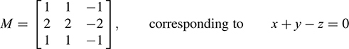
Here u = (1, −1, 0) and υ = (1, 0, 1) are linearly independent solutions.
(ii) Subtract λ = 5 down the diagonal of A to obtain the matrix

Only z is a free variable. Here w = (1, 2, 1) is a solution.
Thus, S = {u, υ, w} = {(1, −1, 0), (1, 0, 1), (1, 2, 1)g} is a maximal set of linearly independent eigenvectors of A.
Remark: The vectors u and υ were chosen so that they were independent solutions of the system x + y − z = 0. On the other hand, w is automatically independent of u and υ because w belongs to a different eigenvalue of A. Thus, the three vectors are linearly independent.
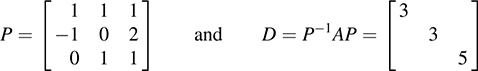
(c) A is diagonalizable, because it has three linearly independent eigenvectors. Let P be the matrix with columns u, υ, w. Then
9.15. Repeat Problem 9.14 for the matrix  .
.
(a) First find the characteristic polynomial Δ(t) of B. We have

Therefore, Δ(t) = t3 − 12t + 16 = (t − 2)2(t + 4). Thus, λ1 = 2 and λ2 = 4 are the eigenvalues of B.
(b) Find a basis for the eigenspace of each eigenvalue of B.
(i) Subtract λ1 = 2 down the diagonal of B to obtain

The system has only one independent solution; for example, x = 1, y = 1, z = 0. Thus, u = (1, 1, 0) forms a basis for the eigenspace of λ1 = 2.
(ii) Subtract λ2 = −4 (or add 4) down the diagonal of B to obtain

The system has only one independent solution; for example, x = 0, y = 1, z = 1. Thus, υ = (0, 1, 1) forms a basis for the eigenspace of λ2 = −4.
Thus S = {u, υ} is a maximal set of linearly independent eigenvectors of B.
(c) Because B has at most two linearly independent eigenvectors, B is not similar to a diagonal matrix; that is, B is not diagonalizable.
9.16. Find the algebraic and geometric multiplicities of the eigenvalue λ1 = 2 of the matrix B in Problem 9.15.
The algebraic multiplicity of λ1 = 2 is 2, because t − 2 appears with exponent 2 in Δ(t). However, the geometric multiplicity of λ1 = 2 is 1, because dim Eλ1 = 1 (where Eλ1 is the eigenspace of λ1).
9.17. Let T: R3 → R3 be defined by T(x, y, z) = (2x + y − 2z, 2x + 3y − 4z, x + y − z). Find all eigenvalues of T, and find a basis of each eigenspace. Is T diagonalizable? If so, find the basis S of R3 that diagonalizes T, and find its diagonal representation D.
First find the matrix A that represents T relative to the usual basis of R3 by writing down the coefficients of x, y, z as rows, and then find the characteristic polynomial of A (and T). We have
Therefore, Δ(t) = t3 − 4t2 + 5t − 2 = (t − 1)2(t − 2), and so λ = 1 and λ = 2 are the eigenvalues of A (and T). We next find linearly independent eigenvectors for each eigenvalue of A.
(i) Subtract λ = 1 down the diagonal of A to obtain the matrix
Here y and z are free variables, and so there are two linearly independent eigenvectors belonging to λ = 1. For example, u = (1, −1, 0) and υ = (2, 0, 1) are two such eigenvectors.
(ii) Subtract λ = 2 down the diagonal of A to obtain

Only z is a free variable. Here w = (1, 2, 1) is a solution.
Thus, T is diagonalizable, because it has three independent eigenvectors. Specifically, choosing

as a basis, T is represented by the diagonal matrix D = diag(1, 1, 2).
9.18. Prove the following for a linear operator (matrix) T:
(a) The scalar 0 is an eigenvalue of T if and only if T is singular.
(b) If λ is an eigenvalue of T, where T is invertible, then λ−1 is an eigenvalue of T−1.
(a) We have that 0 is an eigenvalue of T if and only if there is a vector υ ≠ 0 such that T(υ) = 0 υ—that is, if and only if T is singular.
(b) Because T is invertible, it is nonsingular; hence, by (a), λ ≠ 0. By definition of an eigenvalue, there exists υ ≠ 0 such that T(υ) = λ υ. Applying T−1 to both sides, we obtain

Therefore, λ−1 is an eigenvalue of T−1.
9.19. Let λ be an eigenvalue of a linear operator T: V → V, and let Eλ consists of all the eigenvectors belonging to λ (called the eigenspace of λ). Prove that Eλ is a subspace of V. That is, prove
(a) If u ∈ Eλ, then ku ∈ Eλ for any scalar k. (b) If u, υ, ∈ Eλ, then u + υ ∈ Eλ.
(a) Because u ∈ Eλ, we have T(u) = λu. Then T(ku) = kT(u) = k(λu) = λ(ku), and so ku ∈ Eλ: (We view the zero vector 0 ∈ V as an“eigenvector” of λ in order for Eλ to be a subspace of V.)
(b) As u, υ ∈ Eλ, we have T(u) = λu and T(υ) = λ υ. Then T(u + υ) = T(u) + T(υ) = λu + λ υ = λ(u + υ); and so u + υ ∈ Eλ
9.20. Prove Theorem 9.6: The following are equivalent: (i) The scalar λ is an eigenvalue of A.
(ii) The matrix λI − A is singular.
(iii) The scalar λ is a root of the characteristic polynomial Δ(t) of A.
The scalar λ is an eigenvalue of A if and only if there exists a nonzero vector υ such that

or λI − A is singular. In such a case, λ is a root of Δ(t) = |tI − A|. Also, υ is in the eigenspace Eλ of λ if and only if the above relations hold. Hence, υ is a solution of (λI − A)X = 0.
9.21. Prove Theorem 9.8′: Suppose υ1, υ2, …, υn are nonzero eigenvectors of T belonging to distinct eigenvalues λ1, λ2, …, λn. Then υ1, υ2, …, υn are linearly independent.
Suppose the theorem is not true. Let υ1, υ2, …, υs be a minimal set of vectors for which the theorem is not true. We have s > 1, because υ1 ≠ 0. Also, by the minimality condition, υ2, …, υs are linearly independent. Thus, υ1 is a linear combination of υ2, …, υs, say,

(where some ak ≠ 0). Applying T to (1) and using the linearity of T yields

Because υj is an eigenvector of T belonging to λj, we have T(υj) = λj υj. Substituting in (2) yields

Multiplying (1) by λ1 yields

Setting the right-hand sides of (3) and (4) equal to each other, or subtracting (3) from (4) yields

Because υ2, υ3, …, υs are linearly independent, the coefficients in (5) must all be zero. That is,

However, the λi are distinct. Hence λ1 − λj ≠ 0 for j > 1. Hence, a2 = 0, a3 = 0, …, as = 0. This contradicts the fact that some ak ≠ 0. The theorem is proved.
9.22. Prove Theorem 9.9. Suppose Δ(t) = (t − a1)(t − a2) … (t − an) is the characteristic polynomial of an n-square matrix A, and suppose the n roots ai are distinct. Then A is similar to the diagonal matrix D = diag(a1, a2, …, an).
Let υ1, υ2, …, υn be (nonzero) eigenvectors corresponding to the eigenvalues ai. Then the n eigenvectors υi are linearly independent (Theorem 9.8), and hence form a basis of Kn. Accordingly, A is diagonalizable (i.e., A is similar to a diagonal matrix D), and the diagonal elements of D are the eigenvalues ai.
9.23. Prove Theorem 9.10′: The geometric multiplicity of an eigenvalue λ of T does not exceed its algebraic multiplicity.
Suppose the geometric multiplicity of λ is r. Then its eigenspace Eλ contains r linearly independent eigenvectors υ1, …, υr. Extend the set {υi} to a basis of V, say, {υi, …, υr, w1, …, ws}. We have

Then 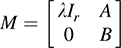 is the matrix of T in the above basis, where A = [aij]T and B = [bij]T:
Because M is block diagonal, the characteristic polynomial (t − λ)r of the block λIr must divide the characteristic polynomial of M and hence of T. Thus, the algebraic multiplicity of λ for T is at least r, as required.
Diagonalizing Real Symmetric Matrices and Quadratic Forms
9.24. Let  . Find an orthogonal matrix P such that D = P−1AP is diagonal.
First find the characteristic polynomial Δ(t) of A. We have

Thus, the eigenvalues of A are λ = 8 and λ = 2. We next find corresponding eigenvectors.
Subtract λ = 8 down the diagonal of A to obtain the matrix

A nonzero solution is u1 = (3, 1).
Subtract λ = −2 (or add 2) down the diagonal of A to obtain the matrix

A nonzero solution is u2 = (1, −3).
As expected, because A is symmetric, the eigenvectors u1 and u2 are orthogonal. Normalize u1 and u2 to obtain, respectively, the unit vectors

Finally, let P be the matrix whose columns are the unit vectors û1 and û2, respectively. Then

As expected, the diagonal entries in D are the eigenvalues of A.
9.25. Let  . (a) Find all eigenvalues of B.
(b) Find a maximal set S of nonzero orthogonal eigenvectors of B.
(c) Find an orthogonal matrix P such that D = P−1BP is diagonal.
(a) First find the characteristic polynomial of B. We have

Hence, Δ(t) = t3 − 6t2 − 135t − 400. If Δ(t) has an integer root it must divide 400. Testing t = −5, by synthetic division, yields
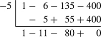
Thus, t + 5 is a factor of Δ(t), and t2 − 11t − 80 is a factor. Thus,

The eigenvalues of B are λ = 5 (multiplicity 2), and λ = 16 (multiplicity 1).
(b) Find an orthogonal basis for each eigenspace. Subtract λ = 5 (or, add 5) down the diagonal of B to obtain the homogeneous system

That is, 4x − 2y + z = 0. The system has two independent solutions. One solution is υ1 = (0, 1, 2). We seek a second solution υ2 = (a, b, c), which is orthogonal to υ1, such that

One such solution is υ2 = (−5, −8, 4).
Subtract λ = 16 down the diagonal of B to obtain the homogeneous system

This system yields a nonzero solution υ3 = (4, −2, 1). (As expected from Theorem 9.13, the eigenvector υ3 is orthogonal to υ1 and υ2.)
Then υ1, υ2, υ3 form a maximal set of nonzero orthogonal eigenvectors of B.
(c) Normalize υ1, υ2, υ3 to obtain the orthonormal basis:

Then P is the matrix whose columns are  . Thus,

9.26. Let q(x, y) = x2 + 6xy − 7y2. Find an orthogonal substitution that diagonalizes q.
Find the symmetric matrix A that represents q and its characteristic polynomial Δ(t). We have

The eigenvalues of A are λ = 2 and λ = 8. Thus, using s and t as new variables, a diagonal form of q is

The corresponding orthogonal substitution is obtained by finding an orthogonal set of eigenvectors of A.
(i) Subtract λ = 2 down the diagonal of A to obtain the matrix

A nonzero solution is u1 = (3, 1).
(ii) Subtract λ = −8 (or add 8) down the diagonal of A to obtain the matrix

A nonzero solution is u2 = (−1, 3).
As expected, because A is symmetric, the eigenvectors u1 and u2 are orthogonal.
Now normalize u1 and u2 to obtain, respectively, the unit vectors

Finally, let P be the matrix whose columns are the unit vectors û1 and û2, respectively, and then [x, y]T = P[s, t]T is the required orthogonal change of coordinates. That is,

One can also express s and t in terms of x and y by using P−1 = PT. That is,

Minimal Polynomial
9.27. Let  and
and  . The characteristic polynomial of both matrices is Δ(t) = (t − 2)(t − 1)2. Find the minimal polynomial m(t) of each matrix.
The minimal polynomial m(t) must divide Δ(t). Also, each factor of Δ(t) (i.e., t − 2 and t − 1) must also be a factor of m(t). Thus, m(t) must be exactly one of the following:

(a) By the Cayley–Hamilton theorem, g(A) = Δ(A) = 0, so we need only test f(t). We have

Thus, m(t) = f(t) = (t − 2)(t − 1) = t2 − 3t + 2 is the minimal polynomial of A.
(b) Again g(B) = Δ(B) = 0, so we need only test f(t). We get

Thus, m(t) ≠ f(t). Accordingly, m(t) = g(t) = (t − 2)(t − 1)2 is the minimal polynomial of B. [We emphasize that we do not need to compute g(B); we know g(B) = 0 from the Cayley–Hamilton theorem.]
9.28. Find the minimal polynomial m(t) of each of the following matrices:
(a) 
(a) The characteristic polynomial of A is Δ(t) = t2 − 12t + 32 = (t − 4)(t − 8). Because Δ(t) has distinct factors, the minimal polynomial m(t) = Δ(t) = t2 − 12t + 32.
0(b) Because B is triangular, its eigenvalues are the diagonal elements 1, 2, 3; and so its characteristic polynomial is Δ(t) = (t − 1)(t − 2)(t − 3). Because Δ(t) has distinct factors, m(t) = Δ(t).
(c) The characteristic polynomial of C is Δ(t) = t2 − 6t + 9 = (t − 3)2. Hence the minimal polynomial of C is f(t) = t 3 or g(t) = (t − 3)2. However, f(C) ≠ 0; that is, C − 3I ≠ 0. Hence,

9.29. Suppose S = {u1, u2, …, un} is a basis of V, and suppose F and G are linear operators on V such that [F] has 0’s on and below the diagonal, and [G] has a ≠ 0 on the superdiagonal and 0’s elsewhere. That is,

Show that (a) Fn = 0, (b) Gn−1 ≠ 0, but Gn = 0. (These conditions also hold for [F] and [G].)
(a) We have F(u1) = 0 and, for r > 1, F(ur) is a linear combination of vectors preceding ur in S. That is,

Hence, F2(ur) = F(F(ur)) is a linear combination of vectors preceding ur−1, and so on. Hence, Fr(ur) = 0 for each r. Thus, for each r, Fn(ur) = Fn−r (0) = 0, and so Fn = 0, as claimed.
(b) We have G(u1) = 0 and, for each k > 1, G(uk) = auk−1. Hence, Gr(uk) = aruk−r for r < k. Because a ≠ 0, an−1 ≠ 0. Therefore, Gn−1 (un) = an−1 u1 ≠ 0, and so Gn−1 ≠ 0. On the other hand, by (a), Gn = 0.
9.30. Let B be the matrix in Example 9.12(a) that has 1’s on the diagonal, a’s on the superdiagonal, where a ≠ 0, and 0’s elsewhere. Show that f(t) = (t − λ)n is both the characteristic polynomial Δ(t) and the minimum polynomial m(t) of A.
Because A is triangular with λ’s on the diagonal, Δ(t) = f(t) = (t − λ)n is its characteristic polynomial. Thus, m(t) is a power of t − λ. By Problem 9.29, (A − λI)r−1 ≠ 0. Hence, m(t) = Δ(t) = (t − λ)n.
9.31. Find the characteristic polynomial Δ(t) and minimal polynomial m(t) of each matrix:
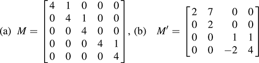
(a) M is block diagonal with diagonal blocks

The characteristic and minimal polynomial of A is f(t) = (t − 4)3 and the characteristic and minimal polynomial of B is g(t) = (t − 4)2. Then

(where LCM means least common multiple). We emphasize that the exponent in m(t) is the size of the largest block.
(b) Here M′ is block diagonal with diagonal blocks  and
and  The characteristic and minimal polynomial of A′ is f(t) = (t − 2)2. The characteristic polynomial of B′ is g(t) = t2 − 5t + 6 = (t − 2)(t − 3), which has distinct factors. Hence, g(t) is also the minimal polynomial of B. Accordingly,

9.32. Find a matrix A whose minimal polynomial is f(t) = t3 − 8t2 + 5t + 7.
Simply let  , the companion matrix of f(t) [defined in Example 9.12(b)].
9.33. Prove Theorem 9.15: The minimal polynomial m(t) of a matrix (linear operator) A divides every polynomial that has A as a zero. In particular (by the Cayley–Hamilton theorem), m(t) divides the characteristic polynomial Δ(t) of A.
Suppose f(t) is a polynomial for which f(A) = 0. By the division algorithm, there exist polynomials q(t) and r(t) for which f(t) = m(t)q(t) + r(t) and r(t) = 0 or deg r(t) < deg m(t). Substituting t = A in this equation, and using that f(A) = 0 and m(A) = 0, we obtain r(A) = 0. If r(t) ≠ 0, then r(t) is a polynomial of degree less than m(t) that has A as a zero. This contradicts the definition of the minimal polynomial. Thus, r(t) = 0, and so f(t) = m(t)q(t); that is, m(t) divides f(t).
9.34. Let m(t) be the minimal polynomial of an n-square matrix A. Prove that the characteristic polynomial Δ(t) of A divides [m(t)n.
Suppose m(t) = tr + c1tr−1 · · · + cr−1t + cr. Define matrices Bj as follows:
Then

Set
Then

Taking the determinant of both sides gives |tI − AjjB(t)| = |m(t)I| = [m(t)]n. Because |B(t)| is a polynomial, |tI − A| divides [m(t)]n; that is, the characteristic polynomial of A divides [m(t)]n.
9.35. Prove Theorem 9.16: The characteristic polynomial Δ(t) and the minimal polynomial m(t) of A have the same irreducible factors.
Suppose f(t) is an irreducible polynomial. If f(t) divides m(t), then f(t) also divides Δ(t) [because m(t) divides Δ(t). On the other hand, if f(t) divides Δ(t), then by Problem 9.34, f(t) also divides [m(t)]n. But f(t) is irreducible; hence, f(t) also divides m(t). Thus, m(t) and Δ(t) have the same irreducible factors.
9.36. Prove Theorem 9.19: The minimal polynomial m(t) of a block diagonal matrix M with diagonal blocks Ai is equal to the least common multiple (LCM) of the minimal polynomials of the diagonal blocks Ai.
We prove the theorem for the case r = 2. The general theorem follows easily by induction. Suppose  , where A and B are square matrices. We need to show that the minimal polynomial m(t) of M is the LCM of the minimal polynomials g(t) and h(t) of A and B, respectively.
Because m(t) is the minimal polynomial of  , and m(A) = 0 and m(B) = 0. Because g(t) is the minimal polynomial of A, g(t) divides m(t). Similarly, h(t) divides m(t). Thus m(t) is a multiple of g(t) and h(t).
Now let f(t) be another multiple of g(t) and h(t). Then  . But m(t) is the minimal polynomial of M; hence, m(t) divides f(t). Thus, m(t) is the LCM of g(t) and h(t).
9.37. Suppose m(t) = tr + ar−1tr−1 + · · · + a1t + a0 is the minimal polynomial of an n-square matrix A. Prove the following:
(a) A is nonsingular if and only if the constant term a0 ≠ 0.
(b) If A is nonsingular, then A−1 is a polynomial in A of degree r − 1 < n.
(a) The following are equivalent: (i) A is nonsingular, (ii) 0 is not a root of m(t), (iii) a0 ≠ 0. Thus, the statement is true.
(b) Because A is nonsingular, a0 ≠ 0 by (a). We have
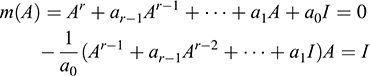
Thus,
Accordingly,
SUPPLEMENTARY PROBLEMS
Polynomials of Matrices
9.38. Let  and
and  . Find f(A), g(A), f(B), g(B), where f(t) = 2t2 − 5t + 6 and g(t) = t3 − 2t2 + t + 3.
9.39. Let  . Find A2, A3, An, where n > 3, and A−1.
9.40. Let  . Find a real matrix A such that B = A3.
9.41. For each matrix, find a polynomial having the following matrix as a root:
9.42. Let A be any square matrix and let f(t) be any polynomial. Prove (a) (P−1AP)n = P−1AnP.
(b)f(P−1AP) = P−1f(A)P. (c) f(AT) = [f(A)]T. (d) If A is symmetric, then f(A) is symmetric.
9.43. Let M = diag[A1, …, Ar] be a block diagonal matrix, and let f(t) be any polynomial. Show that f(M) is block diagonal and f(M) = diag[f(A1), …, f(Ar)]:
9.44. Let M be a block triangular matrix with diagonal blocks A1, …, Ar, and let f(t) be any polynomial. Show that f(M) is also a block triangular matrix, with diagonal blocks f(A1), …, f(Ar).
Eigenvalues and Eigenvectors
9.45. For each of the following matrices, find all eigenvalues and corresponding linearly independent eigenvectors:

When possible, find the nonsingular matrix P that diagonalizes the matrix.
 .
.(a) Find eigenvalues and corresponding eigenvectors.
(b) Find a nonsingular matrix P such that D = P−1AP is diagonal.
(c) Find A8 and f(A) where f(t) = t4 − 5t3 + 7t2 − 2t + 5.
(d) Find a matrix B such that B2 = A.
9.47. Repeat Problem 9.46 for  .
.
9.48. For each of the following matrices, find all eigenvalues and a maximum set S of linearly independent eigenvectors:

Which matrices can be diagonalized, and why?
9.49. Find: (a) 2 × 2 matrix A with eigenvalues λ1 = 1 and λ2 =−2 and corresponding eigenvectors v1 = (1, 2) and v2 = (3, 7).
(b) 3 × 3 matrix A with eigenvalues λ1 = 1, λ2 = 2, λ2 = 3 and corresponding eigenvectors v1 = (1, 0, 1), v2 = (1, 1, 2), v3 = (1, 2, 4). [Hint: See Problem 2.19.]
9.50. Let  be a real matrix. Find necessary and sufficient conditions on a, b, c, d so that A is diagonalizable—that is, so that A has two (real) linearly independent eigenvectors.
9.51. Show that matrices A and AT have the same eigenvalues. Give an example of a 2 − 2 matrix A where A and AT have different eigenvectors.
9.52. Suppose υ is an eigenvector of linear operators F and G. Show that υ is also an eigenvector of the linear operator kF + k′G, where k and k′ are scalars.
9.53. Suppose υ is an eigenvector of a linear operator T belonging to the eigenvalue λ. Prove
(a) For n > 0, υ is an eigenvector of Tn belonging to λn.
(b) f (λ) is an eigenvalue of f(T) for any polynomial f(t).
9.54. Suppose λ ≠ 0 is an eigenvalue of the composition F ° G of linear operators F and G. Show that λ is also an eigenvalue of the composition G ° F. [Hint: Show that G(υ) is an eigenvector of G ° F.]
9.55. Let E: V → V be a projection mapping; that is, E2 = E. Show that E is diagonalizable and, in fact, can be represented by the diagonal matrix  , where r is the rank of E.
Diagonalizing Real Symmetric Matrices and Quadratic Forms
9.56. For each of the following symmetric matrices A, find an orthogonal matrix P and a diagonal matrix D such that D = P−1AP:

9.57. For each of the following symmetric matrices B, find its eigenvalues, a maximal orthogonal set S of eigenvectors, and an orthogonal matrix P such that D = P−1BP is diagonal:

9.58. Using variables s and t, find an orthogonal substitution that diagonalizes each of the following quadratic forms:

9.59. For each of the following quadratic forms q(x, y, z), find an orthogonal substitution expressing x, y, z in terms of variables r, s, t, and find q(r, s, t):

9.60. Find a real 2 − 2 symmetric matrix A with eigenvalues:
(a) λ = 1 and λ = 4 and eigenvector u = (1, 1) belonging to λ = 1;
(b) λ = 2 and λ = 3 and eigenvector u = (1, 2) belonging to λ = 2.
In each case, find a matrix B for which B2 = A.
Characteristic and Minimal Polynomials
9.61. Find the characteristic and minimal polynomials of each of the following matrices:

9.62. Find the characteristic and minimal polynomials of each of the following matrices:
9.63. Let  and
and  . Show that A and B have different characteristic polynomials (and so are not similar) but have the same minimal polynomial. Thus, nonsimilar matrices may have the same minimal polynomial.
9.64. Let A be an n-square matrix for which Ak = 0 for some k > n. Show that An = 0.
9.65. Show that a matrix A and its transpose AT have the same minimal polynomial.
9.66. Suppose f(t) is an irreducible monic polynomial for which f(A) = 0 for a matrix A. Show that f(t) is the minimal polynomial of A.
9.67. Show that A is a scalar matrix kI if and only if the minimal polynomial of A is m(t) = t − k.
9.68. Find a matrix A whose minimal polynomial is (a) t3 − 5t2 + 6t + 8, (b) t4 − 5t3 − 2t + 7t + 4.
9.69. Let f(t) and g(t) be monic polynomials (leading coefficient one) of minimal degree for which A is a root. Show f(t) = g(t): [Thus, the minimal polynomial of A is unique.]
ANSWERS TO SUPPLEMENTARY PROBLEMS
Notation: M = [R1; R2;...] denotes a matrix M with rows R1, R2, ….
9.38. f(A) = [26, −3; 5, −27, g(A) = [40, 39; −65, −27], f(B) = [3, 6; 0, 9], g(B) = [3, 12; 0, 15]
9.39. A2 = [1, 4; 0, 1], A3 = [1, 6; 0, 1], An = [1, −2n; 0, 1], A−1 = [1, −2; 0, 1]
9.40. Let A = [2, a, b; 0, 2, c; 0, 0, 2]. Set B = A3 and then 
9.41. Find Δ(t): (a) t2 + t − 11, (b) t2 + 2t + 13, (c) t3 − 7t2 + 6t − 1
9.45. (a) λ = 1, u = (3, 1); λ = −4, υ = (1, 2), (b) λ = 4, u = (2, 1),
(c) λ = −1, u = (2, 1); λ = 5, υ = (2, 3). Only A and C can be diagonalized; use P = [u, υ].
9.46. (a) λ = 1, u = (1, 1); λ = 4, υ = (1, −2),
(b) P = [u, υ],
(c) f(A) = [3, 1; 2, 1], A8 = [21 846, −21 845; −43 690, 43 691],
(d) 
9.47. (a) λ = 1, u = (3, −2); λ = 2, υ = (2, −1), (b) P = [u, υ],
(c) f(A) = [2, −6; 2, 9], A8 = [1021, 1530; −510, −764],
(d) 
9.48. (a) λ = 2, u = (1, 1, 0), υ = (1, 0, −1); λ = 4, w = (1, 1, 2),
(b) λ = 2, u = (1, 1, 0); λ = 4, υ = (0, 1, 1),
(c) λ = 3, u = (1, 1, 0), υ = (1, 0, 1); λ = 1, w = (2, −1, 1). Only A and C can be diagonalized; use P = [u, υ, w].
9.49. (a) [19, −9; 42, −20], (b) [1, 1, 0; −2, 0, 2; −4, −2, 5]
9.50. We need [tr(A)2 − 4[det(A)] ≥ 0 or (a − d)2 + 4bc ≥ 0.

9.57. (a) λ = 1, u = (1, −1, 0), υ = (1, 1, −2); λ = 2, w = (1, 1, 1),
(b) λ = 1; u = (2, 1, −1), υ = (2, −3, 1); λ = 22; w = (1, 2, 4);
Normalize u, υ, w, obtaining  , and set
  . (Remark: u and υ are not unique.)


(b) 


9.61. (a) Δ(t) = m(t) = (t − 2)2(t − 6),
(b) Δ(t) = (t − 2)2(t − 6), m(t) = (t − 2)(t − 6)
9.62. (a) Δ(t) = (t − 2)3(t − 7)2, m(t) = (t − 2)2(t − 7),
(b) Δ(t) = (t − 3)5, m(t) = (t − 3)3,
(c) Δ(t) = (t − 2)2(t − 4)2(t − 5); m(t) = (t − 2)(t − 4)(t − 5)
9.68. Let A be the companion matrix [Example 9.12(b)] with last column: (a) [8, −6, 5]T, (b) [4, −7, 2, 5]T
9.69. Hint: A is a root of h(t) = f(t) − g(t), where h(t) − 0 or the degree of h(t) is less than the degree of f(t):