IN THIS CHAPTER, I WILL SHOW YOU how to build two robotic arms, each with its own features and capabilities. You can choose to build one or both depending on your desires and your interest in this topic. However, I will begin the chapter with a reasonably detailed discussion on how robotic arms are defined and designed because that will help you to establish a useful comprehension of this interesting topic.
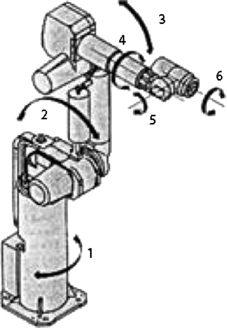
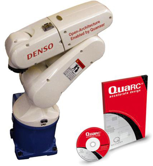
Robotic arms are used extensively in many industrial applications in manufacturing operations. Knowing the basic principles underlying how these arms work will assist you in evaluating when it is appropriate to use this type of robot. Figure 9-1 shows an advanced Denso robotic arm that has 6 degrees of freedom (DOFs), enabling it to perform many intricate operations.
Figure 9-1 Advanced Denso robotic arm.
Understanding robotic arms requires you to know the basic terms and definitions used in this field. The following terms and definitions were sourced from the Society of Robotics website (www.roboticssociety.org ).
Degrees of freedom (DOF) refer to the ability of an arm joint to move in a particular motion. Normally, 1 DOF relates directly to one joint. Therefore, a 3-DOF arm will require three joints. Each joint normally requires one motor and one embedded encoder. Figure 9-2 shows how joints perform 6 DOFs in a robotic arm.
Figure 9-2 6-DOF robotic arm.
Joint motion also may have translation , which is a straight-line or rectilinear motion. The type of motion involved depends on the type of arm attached to the joint.
A free-body diagram (FBD) is often used with the Denavit-Hartenberg (DH) Convention to depict joint motion in both translation and rotation. Figure 9-3 shows a Denso 4-DOF robotic arm with a DH overlay.
Figure 9-3 Free-body robotic arm with DH joint designations.
Please note that links are also shown on the FBD. Link lengths are important in that they form a moment arm, which will have a significant effect on motor loading and performance. Also, joints may have multiple DOFs with essentially zero-length links. Consider your shoulder as an example: it has a multiple range of movement without noticeable links. The human shoulder could be described as a joint with a 3-DOF motion range.
Robot designers often create industrial arm systems use the DH Convention along with FBDs. Such systems typically involve significant forces and are intended for heavy-duty industrial applications. This chapter’s project has no such requirement and thus will not require a DH analysis.
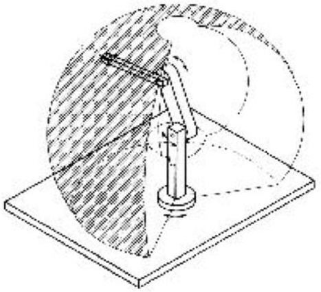
Workspace is the volume of space circumscribed by the robot arm’s maximum range of motion. Figure 9-4 shows the workspace for the robot in Figure 9-3 .
Figure 9-4 Workspace volume.
Workspace volume typically is closely controlled and posted because personnel entering anywhere in this space could be struck and seriously injured by an operating robotic arm. It is also important to ensure that a robotic arm can extend to all points that need to be reached for the particular manufacturing operation that is being automated. It wouldn’t make much sense to have a painting robotic arm that couldn’t quite completely apply paint to the product being manufactured. Ensuring adequate coverage and reach is the responsibility of the project manager in charge of installation of the robotic system.
There are also three broad categories for classifying robotic arms.
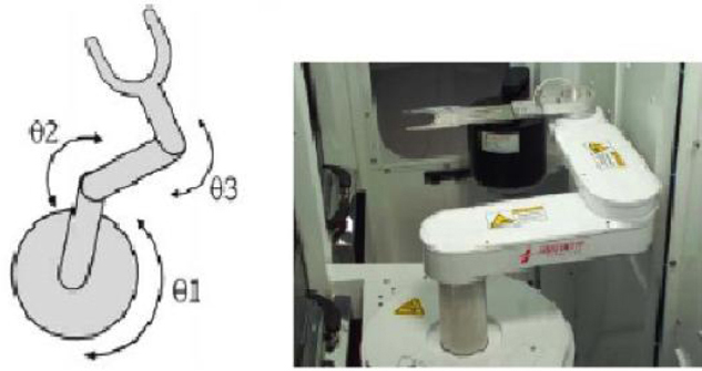
A selectively compliant articulated robot arm (SCARA) is a type of robotic arm that has a very wide range of rotary joint motion. There is a maximum of 620° of joint rotation for the SCARA-compliant robotic arm shown in Figure 9-5 . This wide range of motion is quite remarkable when you consider that typical robotic arm joint motion is 180° or less.
Figure 9-5 SCARA robotic arm.
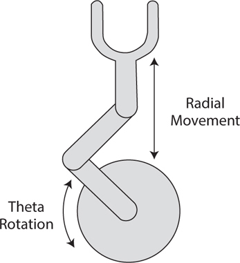
The radial-theta angle (R-Theta ) robotic arm is a more traditional design with more limited joint rotary motion than a SCARA type. The R-Theta also has a linear (radial) placement parameter. Any required linear motion for the end-effector position is automatically computed by the robot controller and is translated to appropriate joint rotary motion. Figure 9-6 illustrates an R-Theta robotic arm.
Figure 9-6 R-Theta robotic arm.
The end-effector position for the X-Y-Z coordinate (Cartesian Coordinate) robotic arm is specified as a set of x , y , and z coordinate positions. The robot controller automatically translates an x-y-z coordinate pair to appropriate joint motion to move the end-effector to the desired position. Figure 9-7 shows a two-dimensional x-y coordinate robot arm. The z direction would be into or out of the plane of the page.
Figure 9-7 X-Y-Z Coordinate robotic arm.
Linear motion was mentioned several times in the preceding descriptions of the various robotic arms. A question you might ask yourself is how linear motion can be accomplished when only rotary joints are being used? The answer is quite simple, and Figure 9-8 shows how it is done.
Figure 9-8 Rotary-to-linear motion conversion.
Suppose that you want to have point T1 travel straight down for a given distance. Imagine commanding a motor at joint J2 to rotate counterclockwise (CCW) for some angular rotation. Point T1 also will move, but it will move in a slight curvilinear direction owing to the angular motion of J2. To counteract this curving motion, joint J1 must be rotated in a clockwise (CW) direction for some angular rotation. The exact CCW rotation for J2 and CW for J1 are computed on a real-time basis by the robotic controller integrated into the arm. The mathematics involved consists of purely trigonometric functions and is a bit tedious—something ideal for a computer to handle.
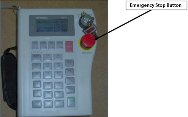
Positioning a robotic arm effector to perform whatever action it has to do, such as welding an auto body seam or painting a body panel, is critical to the overall success of the robot. The process of positioning is called training , and it may be accomplished in several ways. One common way is to manually position the effector and then press a button to record the spatial location as x , y , and z coordinates. Figure 9-9 shows a typical control pendant used to manually position a robotic arm as well as record the incremental positions. The complete path is eventually recorded as a series of points that are then used by the arm controller to smoothly control the robotic arm in its autonomous operation.
Figure 9-9 Teaching pendent.
The robot programmer also will use the controller to make small adjustments to refine the path and to modify the speed of the effector for both safety and product quality assurance. It is very important to have the correct effector speed as a weld is being placed or paint is applied. The robotic arms used in this chapter do not use teaching pendants because such devices are used only in expensive industrial robotic arms.
This completes the introductory discussion. It is now time to show you this chapter’s robotic arms.
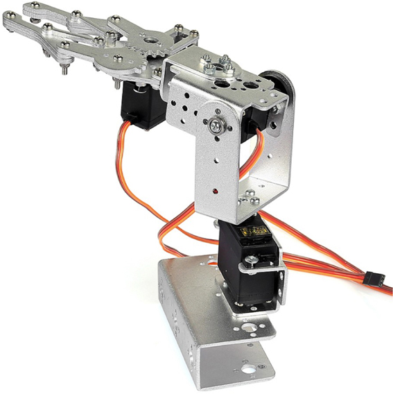
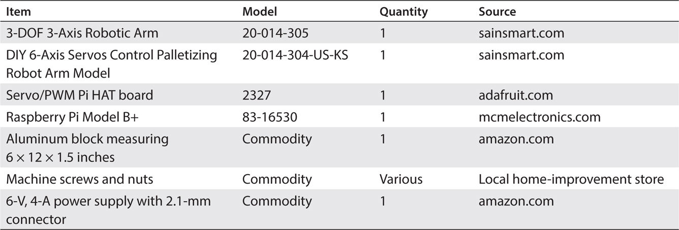
I decided to use two robotic arms to demonstrate the concepts presented in this chapter. Both are distributed by SainSmart, with one being a 3-DOF system with a gripper mechanism and the other a 6-DOF system without a gripper. I chose these two systems to allow you the opportunity to experiment with an actual robotic arm, but one that you could afford. The 3-DOF arm costs about one-fourth as much as the 6-DOF arm. Obviously, the 6-DOF arm offers more flexibility in positioning, but the fundamental concepts underlying these arms are the same. I strongly recommend that you purchase the 3-DOF system and play around with it to see whether your results warrant the additional expense of purchasing the 6-DOF arm. I discuss each of these arms in the next two sections.
Figure 9-10 shows the simpler of the two SainSmart robotic arms I chose as project demonstrators. It is a 3-DOF arm with a gripper assembly, which accounts for one of the DOFs. SainSmart calls its DOFs axes , but they are synonymous.
Figure 9-10 3-DOF SainSmart 3-Axis Robotic Arm.
The precise name of this robotic arm is the SainSmart DIY 3-Axis Servos Control Palletizing Robot Arm Model for Arduino UNO MEGA2560, Item # 20-014-305. Some of the key technical specifications are listed in Table 9-1 .
TABLE 9-1 SainSmart 3-Axis Robotic Arm Key Technical Specifications

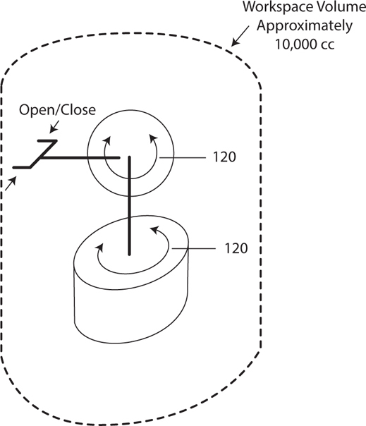
Figure 9-11 shows the rotary-motion range for each joint as well as the total volumetric workspace for the arm.
Figure 9-11 SainSmart 3-DOF arm joint rotary range of motion and volumetric workspace diagram.
It was a bit surprising to see that there was a fairly large volume of 9692 cm3 (0.009692 m3) swept through 120° by the arm when fully extended. This really doesn’t present a safety hazard because the robotic arm is made of acrylonitrile butadiene styrene (ABS), rotates fairly slowly, and uses low forces for both joint and segment motion.
This SainSmart arm uses MG995 servos to operate the two rotary joints and gripper mechanism. These servos are limited to ±60° range of motion for a total range of 120°. These servos are fairly fast and use metal gears for reliable operation. They also use standard servo control signals, which will be discussed in the software section.
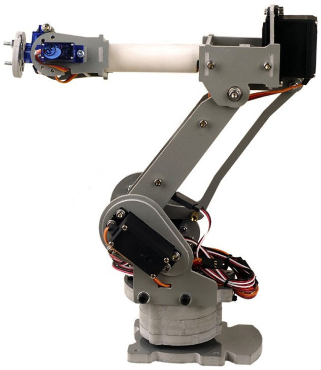
Figure 9-12 shows the SainSmart 6-DOF robotic arm. It is not equipped with a gripper mechanism, as is the 3-DOF arm.
Figure 9-12 6-DOF SainSmart robotic arm.
This arm has more than twice the number of joints as the 3-DOF arm and thus is much more flexible in positioning within its workspace. The arm can lean, which is not possible with the 3-DOF arm, whose main vertical segment is fixed in a single vertical plane. The precise name of this robotic arm is the SainSmart DIY 6-Axis Servos Control Palletizing Robot Arm Model for Arduino UNO MEGA2560, Item # 20-014-304-US-KS. Some of the key technical specifications are listed in Table 9-2 .
TABLE 9-2 SainSmart 6-Axis Robotic Arm Key Technical Specifications
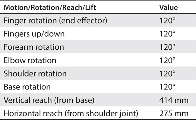
The volumetric workspace is substantially more than that of the 3-DOF arm. I estimated the volume to be approximately 49,748 cm3. It is very difficult to compute the workspace volume because of the many joints in the arm, which means that arm positioning is quite variable. I settled on using a volume that is one-sixth of a sphere with a 414-mm radius. This is very much an overestimate, but it is better to be conservative than compromise this important safety criterion.
In the next section, I discuss a servo control board, which is an essential component between the RasPi and the robotic arms.
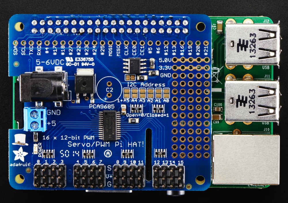
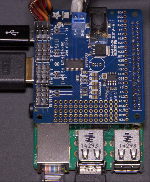
I used the Adafruit 16-Channel PWM/Servo HAT for Raspberry Pi, Minikit # 2327, as a servo control interface board connected between the RasPi and the robotic arm. This control board is shown in Figure 9-13 mounted on a RasPi Model B+.
Figure 9-13 16-Channel PWM/Servo HAT board.
Each of the three robotic arm servos plugs directly into one of the three pin terminal strips mounted on the board. A power supply rated to handle all the attached servos also must be plugged into the control board. I used a 5-V, 4-A supply, which should be more than adequate to power all the servos for either of the robotic arms used in this chapter’s projects.
One distinct advantage of using this particular interface board is its ability to control up to 16 channels of PWM/servo. The RasPi only has two built-in PWM channels, which is quite limiting and would not be sufficient to control either one of the two robotic arms used in this chapter. The interface board makes use of an I2C-controlled PWM controller chip to drive the onboard 16 channels. It is even possible to connect up to 62 additional interface boards in a parallel multidrop I2C network to control an astounding 992 PWM/servo channels. What is even more impressive is that the RasPi’s computational requirement is minimal and totally independent of the number of servos being controlled. Each interface board continually controls the servos plugged into it based on the last I2C commands sent to the board by the RasPi. The RasPi does not have to continually refresh any digital servo control signals, which minimizes its computational burden and frees up the RasPi to handle other important real-time tasks.
At this point in the discussion, I would like to offer you an opportunity to gain some knowledge regarding how the servos function in this robotic arm. I do this in the form of the following sidebar, which is purely optional and will not matter for successful project completion if you choose to skip reading it.
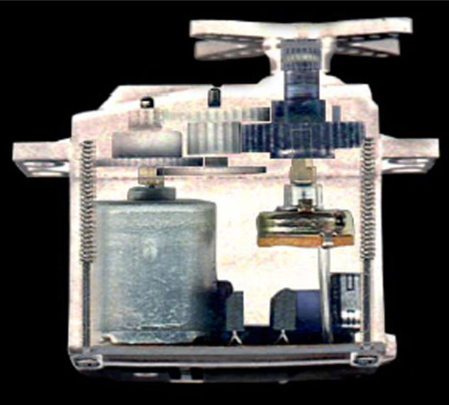
Figure 9-14 is a somewhat transparent view of the inner workings of a standard analog radio-controlled (R/C) servo motor.
Figure 9-14 Inner view of a standard R/C servo motor.
I would like to point out five components in this figure:
 Brushed electric motor (left side).
Gear set (just below the case top).
Servo horn (attached to a shaft protruding above the case top).
Feedback potentiometer (at the bottom end of the same shaft with the horn).
Control PCB (b
ottom on the case to the motor’s right).
The electric motor is just an inexpensive ordinary motor that probably runs at approximately 12,000 rpm unloaded. It typically operates in the 2.5- to 5-VDC range and likely uses less than 200 mA even when fully loaded. The servo torque advantage results from the motor spinning the gear set such that the resulting speed is reduced significantly, producing a very large torque increase compared with the motor’s ungeared rating. A typical motor used in this servo class might have a 0.1 oz-inch torque rating, while the servo output torque could be about 42 oz-inches, which is a 420 times increase in torque production. Of course, the speed would be reduced by the same proportional amount going from 12,000 rpm to about 30 rpm. This slow speed is still sufficiently fast to move the servo shaft to meet normal R/C requirements.
The feedback potentiometer attached to the bottom of the output shaft is a key element in positioning the shaft in accordance with the pulses being received by the servo electronic control board. You may clearly see the feedback potentiometer in Figure 9-15 , which is another image of a disassembled servo.
Figure 9-15 Disassembled servo showing the feedback potentiometer.
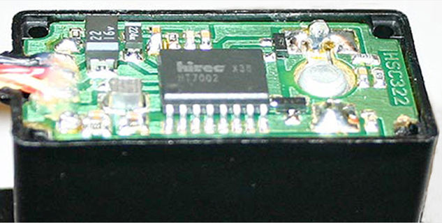
I will discuss the potentiometer’s function further during the control board discussion. The electronics board is the heart of the servo and controls how the servo functions. I will describe an analog control version because that is by far the most popular type used in low-cost servo motors. Figure 9-16 shows a Hitec control board that is in place for its Model HS-311, which is a very common and inexpensive analog servo.
Figure 9-16 Hitec HS-311 electronics board.
The main chip is labeled HT7002, which is a Hitec private model number as well as I could determine. I believe that this chip functions the same as a commercially available chip manufactured by Mitsubishi with Model # M51660L. I will use the M51660L as the basis of my discussion because it is used in a number of other manufacturers’ servo motors and is representative of any chip used in this situation. The Mitsubishi chip is called a Servo Motor Controller for Radio Control, and its pin configuration is shown in Figure 9-17 .
Figure 9-17 Mitsubishi M51660L pin configuration.
Don’t be put off by the different physical configuration between the HT7002 in Figure 9-16 and the chip outline in Figure 9-17 because it is often the case that identical chip dies are placed in different physical packages for any number of reasons. The M51660L block diagram shown in Figure 9-18 illustrates the key functional circuits incorporated into this chip.
Figure 9-18 M51660L block diagram.
Next, I will provide an analysis that will go hand in hand with the demonstration circuit in Figure 9-19 that was provided in the manufacturer’s datasheet (as were the preceding two figures).
Figure 9-19 Demonstration M51660L schematic.
This analysis should help you to understand how an analog servo functions and why there are certain limitations inherent in its design:
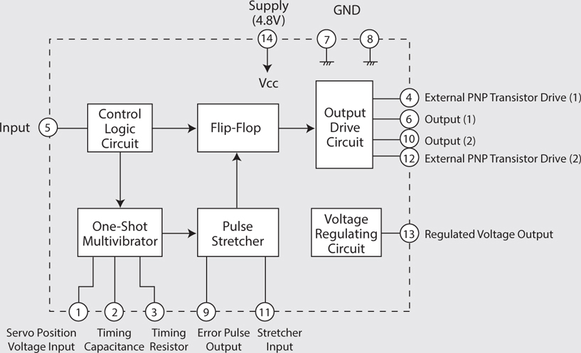
1. The start of a positive pulse appearing on the input line (pin 5) turns on the R-S flip-flop and also starts the one-shot multivibrator running.
2. The R-S flip-flop works in conjunction with the one-shot multivibrator to form a linear one-shot or monostable multivibrator circuit whose on time is proportional to the voltage appearing from the tap on the feedback potentiometer and the charging voltage from the timing capacitor attached to pin 2.
3. The control logic starts comparing the input pulse to the pulse being generated by the one-shot multivibrator.
4. This ongoing comparison results in a new pulse called the error pulse that is than fed to the pulse stretcher and deadband and trigger circuits.
5. The pulse stretcher output ultimately drives the motor control circuit that works in combination with the directional control inputs that originate from the R-S flip-flop. The trigger circuits enable the PNP transistor driver gates for a time period directly proportional to the error pulse.
6. The PNP transistor drive gate outputs are pins 4 and 12, which control two external PNP power transistors that can provide over 200 mA to power the motor. The M51660L chip can only provide up to 20 mA without using these external transistors. This is too little current flow to power the motor in the servo. The corresponding current sinks (return paths) for the external transistors are pins 6 and 10.
7. The 560-kΩ resistor (R f ) connected between pin 2 and the junction of one of the motor leads and pin 6 feeds the motor’s back electromotive force (EMF) voltage into the one-shot multivibrator. Back EMF is created within the motor stator winding when the motor is coasting or when no power pulses are being applied to the motor. This additional voltage input results in a servo damping effect , meaning that it moderates or lessens any servo overshoot or in-place dithering.
This analysis, while a bit lengthy and detailed, was provided to give you an understanding of the complexity of what is constantly happening within the servo case. This knowledge should help you to determine what might be happening if one of your servos starts operating in an erratic manner.
The word deadband was mentioned in step 4, and it is worth some more explanation. Deadband used in this context refers to a slight voltage change in the control input, which should not elicit an output. This is a deliberate design feature: basically, you do not want the servo to react to any slight input changes. Using a deadband improves servo life and makes it less jittery during normal operations. The deadband is fixed in the demonstration circuit by a 1-kΩ resistor connected between pins 9 and 11. This resistor forms another feedback loop between the pulse stretcher input and output.
The last servo parameter I will discuss is the pulse stretcher gain, which largely controls the error pulse length. This gain in the demonstration circuit is set by the values of the capacitor from pin 11 to ground and the resistor connected between pins 11 and 13. This gain would also be referred to as the proportional gain (Kp ) in closed-loop control theory. It is important to have the gain set to what is sometimes jokingly called the “Goldie Locks region”—not too high nor too low, but just right. Too much gain makes the servo much too sensitive and possibly could lead to unstable oscillations. Too little gain makes it too insensitive with a very poor time response. Sometimes experimenters will tweak the resistor and capacitor values in an effort to squeeze out a bit more performance from a servo, but I believe that the manufacturers already have set the component values for a good compromise between performance and stability.
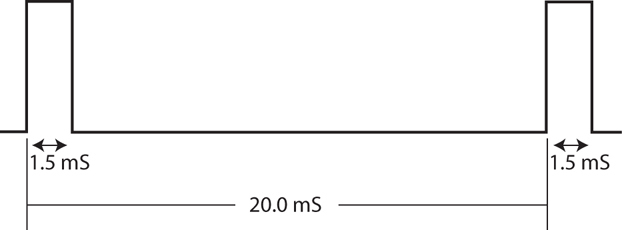
Understanding how digital pulses control an analog servo is the key to knowing how to program it. A series of pulses on the servo signal line with widths of 1.5 ms and a frequency of 50 Hz will cause the servo to remain stationary at its center rotation point. Figure 9-20 illustrates this pulse train.
Figure 9-20 50-Hz, 1.5-ms pulse train.
A 50-Hz frequency is commonly used for these kinds of analog servos, and the pulse amplitude is typically 5 V. The servo will rotate to its full CW rotation position when the pulse width is increased to 2.0 ms. Similarly, the servo will rotate to its full CCW rotation position when the pulse width is decreased to 1.0 ms. Consequently, changing the pulse width from 1.0 to 2.0 ms will cause the servo to move its shaft through its entire range of motion. You also should note that the pulse widths do vary with different servos. In some very inexpensive servos, the range can be from 0.5 to 2.4 ms, while in some pricier ones the range is 0.9 to 2.1 ms. My recommendation is that you check the technical specifications for the servo you will use in your application and adjust the pulse widths appropriately. I would recommend using the website www.servodatabase.com to retrieve the data on your particular servo.
The software controlling the servo is required to generate the pulse width corresponding to the commanded position for the servo rotation angle. I will examine this requirement in further detail in the next section, which discusses the software.
The servo interface control board is controlled by a RasPi using the I2C bus, as was mentioned in my introduction to the interface board. The Wheezy Raspian Linux distribution must be configured to use the I2C bus. The configuration starts with enabling I2C using the raspi-config application. Enter the following to start this config process:
![]()
Select the Advanced Options and then select the Enable I2C option. Next enter
![]()
You next have to install the Python library, which allows you to program the I2C bus. Follow these two steps to install and configure the required software:
1.
sudo apt-get install python-smbus
2.
sudo apt-get install i2c-tools
Using the nano editor, add these two lines to the file /etc/modules:
Use the nano editor to see whether the file /etc/modprobe.d/raspi-blacklist.conf has the following line, and if so, comment it out by placing a number symbol (#
) at the front of the line:
![]()
Using the nano editor, add these two lines to the file /boot/config.txt:

Then:
![]()
Check for all installed I2C devices by entering:
![]()
or:
![]()
(for very early RasPi models).
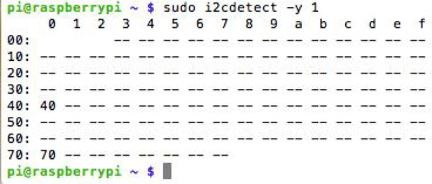
Figure 9-21
shows the result of the i2cdetect
command, which I ran on the RasPi with the 16-channel PWM/Servo HAT module installed.
Figure 9-21
i2cdetect
command result.
The 0x40 address shown comes from the PCA9685 chip on the HAT board. This means that the RasPi is in proper communication with the HAT board using the I2C bus and ready to be programmed, as discussed in the next section.
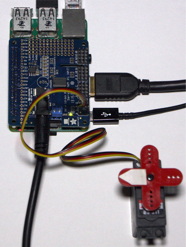
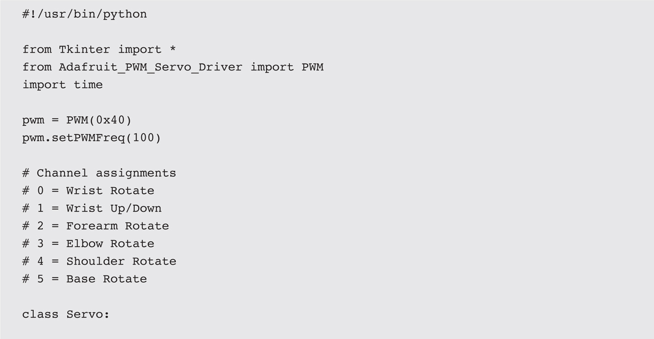
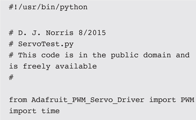
I created a very simple test program named ServoTest.py that exercises a standard Hitec HS-311 servo connected to channel 0 on the HAT board. Figure 9-22 shows the test setup with the servo being powered from a supply connected to the 2.1-mm barrel connector on the HAT board.
Figure 9-22 Initial servo test setup.
The commented ServoTest.py program is listed next and is also available from this book’s companion website.
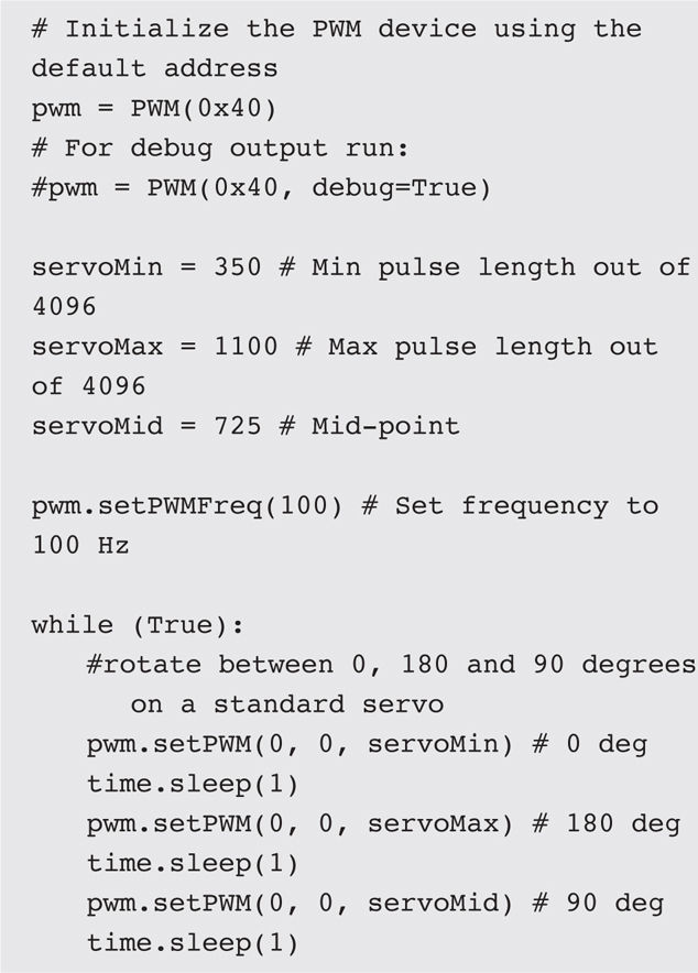
Please note that I set the PWM frequency to 100 Hz versus the normal 50 Hz I mentioned in my servo discussion. This was done purely for convenience sake to ease the pulse-length calculations. The increased frequency has absolutely no effect on the servo’s performance.
I observed that when I ran the program, the servo smoothly rotated between the 0, 180, and 90° positions without any issues. This test confirmed that the RasPi/HAT board was properly configured and ready to handle the robotic arms. Satisfied that I could successfully control a servo, I started the next task of creating a program designed to control all the servos in a robotic arm. It is now time to discuss the software that I created to control the robotic arms.
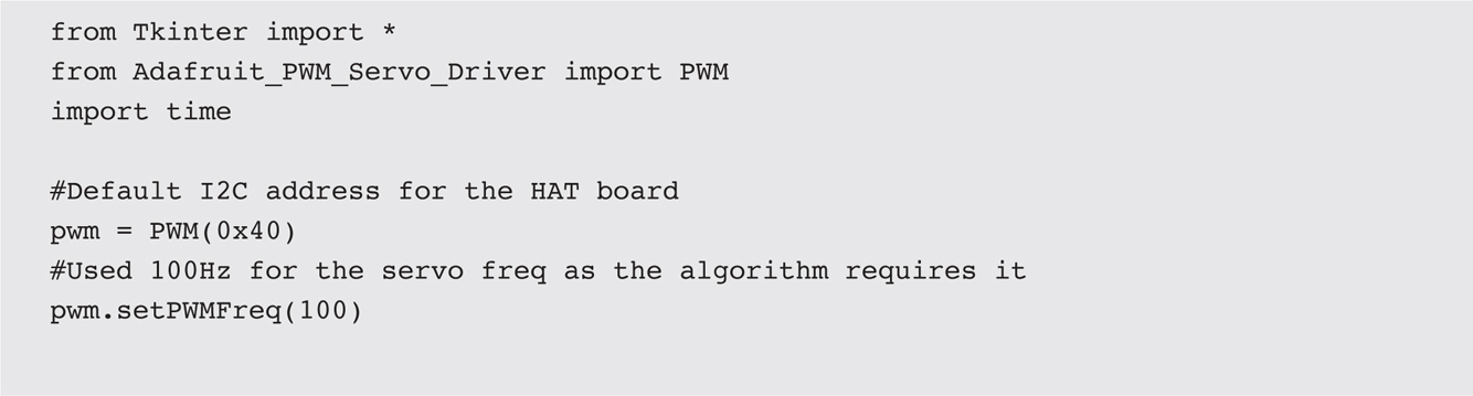
I decided to take a measured approach to developing the robotic arm control software and first try it out with a stand-alone servo as I did with the initial test. In this way, I could resolve any problems that appeared without damaging an expensive robotic arm. I also chose to use a graphical user interface (GUI) for the robotic arm program because such a program naturally lends itself to the way a user would interact with the arm. The GUI was created using the Tkinter library, which is part of the normal Python distributions, including versions 2.7 and 3.0. The arm program also must be run in the X Windows environment because it is a GUI and requires X Windows to correctly display the GUI window and widgets.
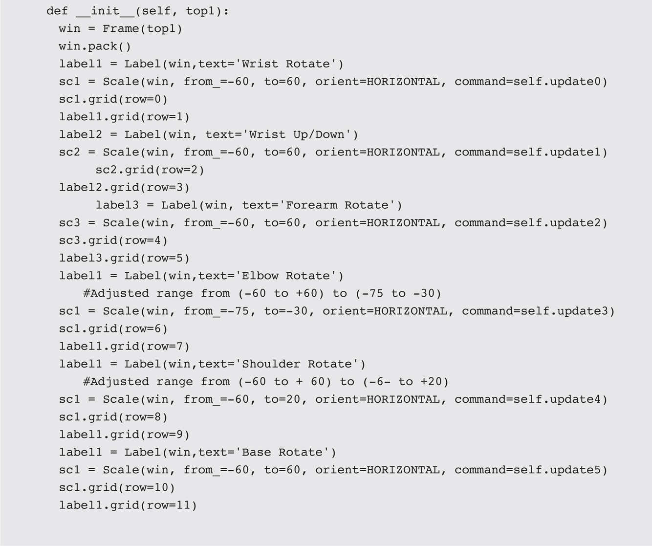
The first arm control program named 3DOF_Robot_Arm.py was created for the 3-DOF arm because that arm uses only three servos, and naturally, such a program would be easier to develop and test. The listing is shown next with a heavy dose of comments included within the code. The source code is also available on this book’s companion website.
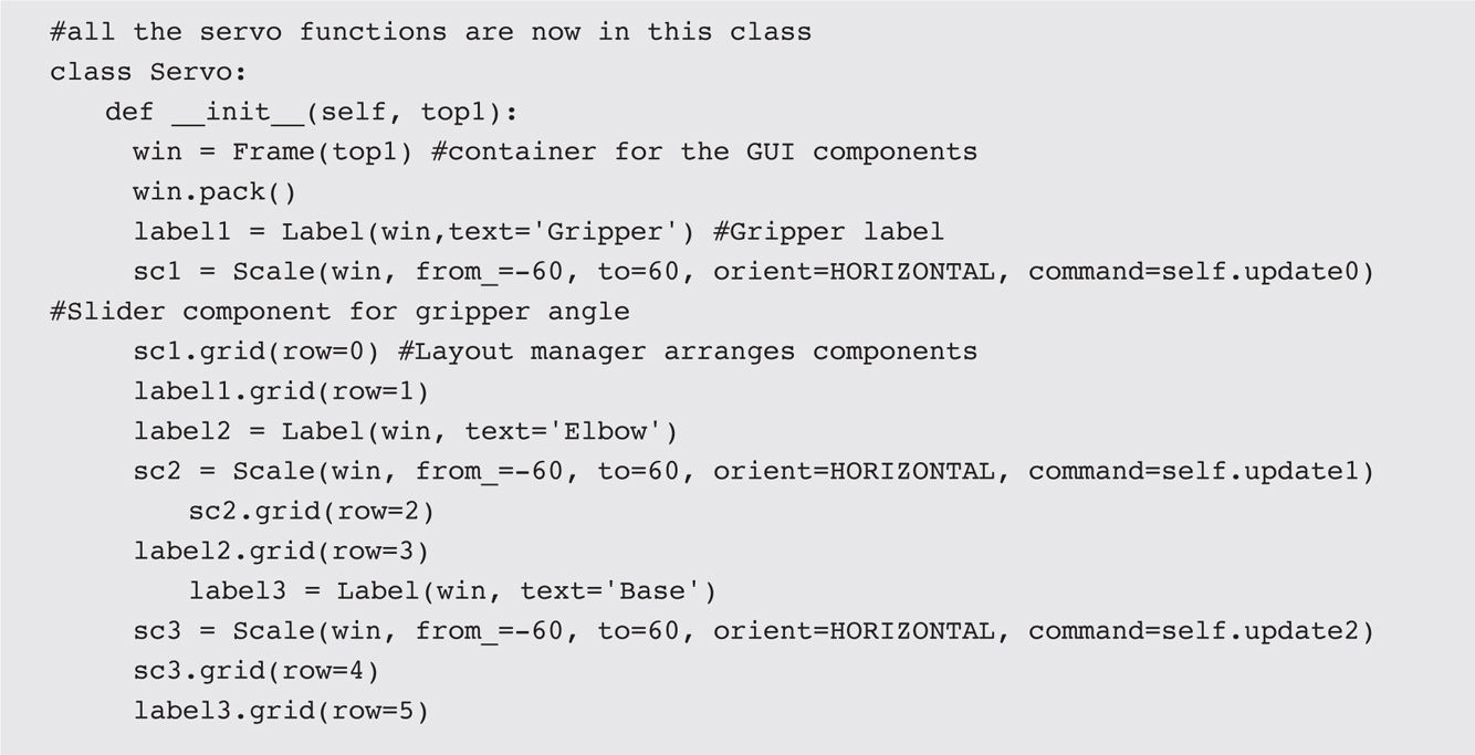
The program is started by first going to the directory, which contains both the 3DOF_Robot_Arm.py and the Adafruit_PWM_Servo_Driver library. You will get an error if you attempt to run the arm program without the library being present in the same directory. The command to cd into the directory containing the 3DOF_Robot_Arm.py and the Adafruit driver library from the home directory is shown next:
Once in the directory, enter these two commands to start X Windows and run the arm program:

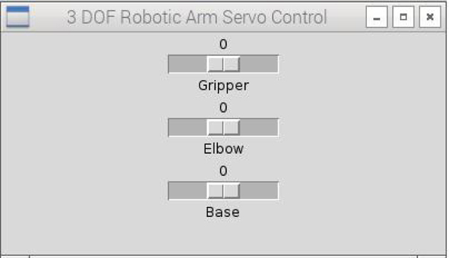
Figure 9-23 is a screenshot of the GUI showing the three labeled slider controls.
Figure 9-23 Robot_Arm program GUI.
Changing the slider position on each of the slider GUI widgets changes the digital pulse width being sent to the HAT servo channel corresponding to the slider widget being changed. The pulse width is 1.0 ms when the slider is at the –60 position and is 2.0 ms when the slider is at the +60 position. The pulse width is 1.5 ms when the slider is at 0, or midway between –60 and +60.
Before running this program with the arm, you must ensure that all the servo leads from the arm have been labeled properly. I identified the lead connections by running the program and then connecting one lead at a time to channel 0. I then moved the slider for the gripper and observed which servo moved. This procedure quickly identified the leads, and I used a label maker to tag the leads. This procedure is not really critical for the 3-DOF robotic arm because the servo leads are easy to identify by visually inspecting the arm. However, the 6-DOF arm has its leads woven all through the structure, making physical lead identification impossible. Besides, identifying the leads using the program also checks the physical connections early in the testing phase and will quickly identify any electrical connection issues. Once all the leads are labeled, you should connect them to the HAT board, as shown in Table 9-3 .
TABLE 9-3 3-DOF Servo Lead Connections
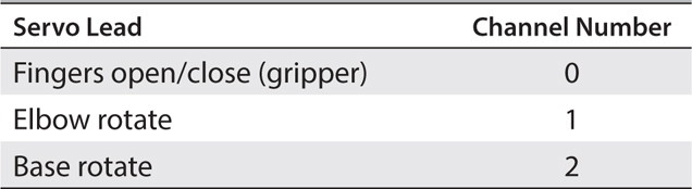
Figure 9-24 shows all the servo leads connected to the HAT board, which, in turn, is mounted on a RasPi.
Figure 9-24 3-DOF servo leads connected to HAT board.
You must clamp the robotic arm to a tabletop before using it. I used a small bar clamp to secure the arm to my worktable. I then tested the 3-DOF robotic arm by running a common industrial robot operation known as pick-and-place . This operation requires the arm to pick up an object and transport it to a different location all within the robot’s volumetric workspace. I used a small wooden block as the transported object. The pick-and-place operation is detailed in the following step sequence:
1. Place the object to be picked up within the reach of the 3-DOF arm.
2. Ensure that the gripper is open and the elbow is rotated to clear the top of the object.
3. Rotate the base such that the gripper opening is centered on the object.
4. Rotate the elbow until the gripper is at the midpoint of the object.
5. Close the gripper to the point where it securely holds the object.
6. Rotate the elbow to lift the object above the mount plane.
7. Rotate the base until it is at the drop-off location.
8. Rotate the elbow until the object rests on the mount surface.
9. Open the gripper to free the object.
10. Rotate the elbow until the gripper is clear of the object.
11. Repeat steps 1 to 10 for additional objects to be moved.
Conveyers also could be required to both deliver objects to be picked as well as to whisk away the objects placed (dropped off). Of course, in a real-world scenario, the robotic arm would be controlled by a real-time program without human intervention. There also would be sensors in place to signal when the object to be picked up was properly arranged and also to signal when the object was dropped off. Development of these real-time programs is normally the topic of robotics courses, where all the ramifications of robotic arm control can be explored.
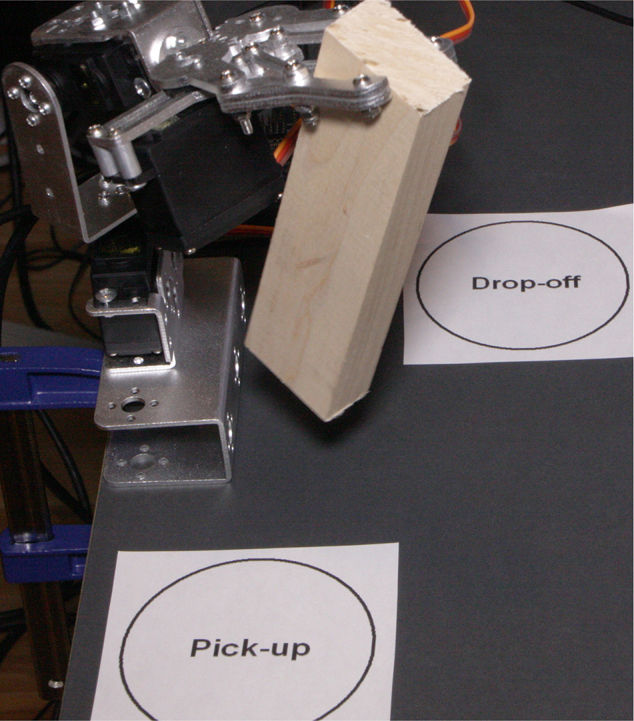
Figure 9-25 shows the 3-DOF robotic arm with an object in its gripper midway between the pick-and-place locations.
Figure 9-25 3-DOF robotic arm in a pick-and-place configuration.
It took me about 20 seconds to manually complete the pick-and-place operation. I would estimate that an automated pick-and-place likely would take no more than 2 seconds, which is a 10 times improvement over manual mode.
Now it is time to examine the 6-DOF arm. I will try a slightly different operational approach with this arm because it significantly more flexible in its positioning owing to the 6 DOFs.
The control program for the 6-DOF arm is named 6DOF_Robot_Arm.py and is listed next. I have not included all the same comments as were in the 3 DOF program because they are all identical. Essentially, the 6-DOF program is simply an extension of the 3-DOF program with three servo control channels added to accommodate the extra DOFs.
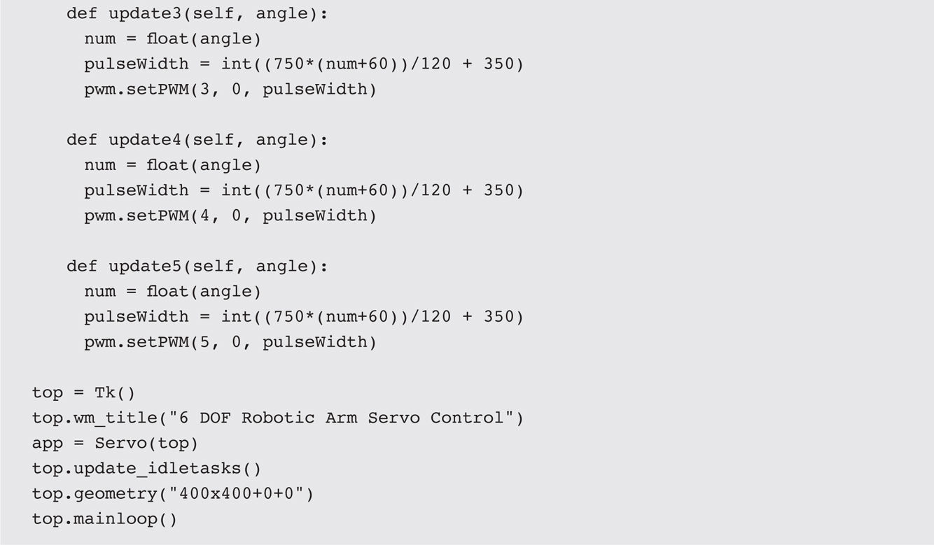
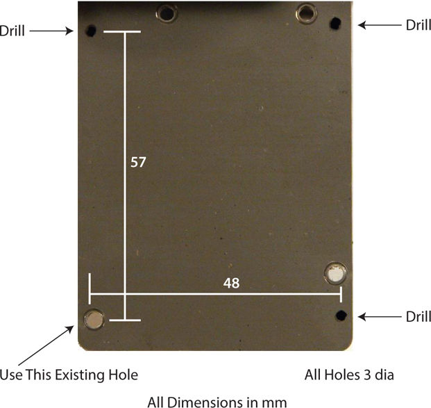
A microcontroller mounting plate is included on this arm because of the large number of servo leads, which potentially could limit the base rotation of the arm. This mounting plate comes with four standoffs placed to support an Arduino Mega 2560 board. I removed these standoffs and drilled three holes to accommodate a RasPi 2 Model B. I also reused one of the existing holes, as shown in Figure 9-26 .
Figure 9-26 Hole placement for a RasPi on the 6-DOF robotic arm mount plate.
I next mounted the RasPi onto the four repositioned standoffs. I would also recommend that you defer connecting the HAT to the RasPi until you complete the servo lead identification procedure.
You must next ensure that all the servo leads from the arm have been labeled properly. Please use the procedure that I detailed in the preceding section to label all the leads. Once all the leads are labeled, you should connect them to the HAT board, as detailed in Table 9-4 .
TABLE 9-4 6-DOF Servo Lead Connections

Connect the whole assembly to the RasPi once all the servo leads are connected to the HAT board. You are now almost ready to test this arm. The arm must be attached to a secure base or platform before operating it because it will fall over if it is extended beyond its stable center of gravity (CG). I will show you the base I used in the next section.
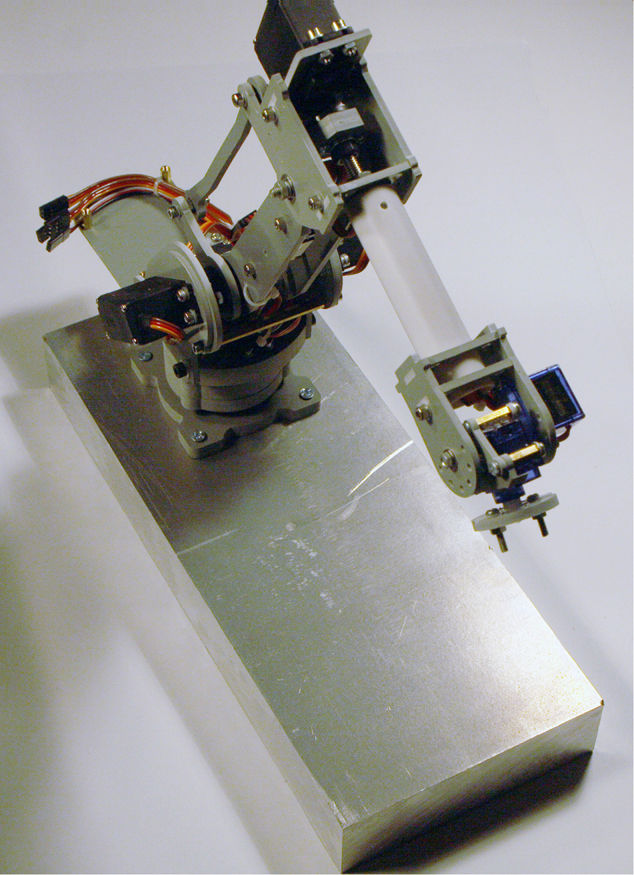
The platform I used was a solid block of aluminum measuring 6 × 12 × 1.5 inches. I drilled and tapped out four mounting holes in the block that matched the mounting holes already drilled in the robotic arm’s mounting plate. The aluminum block weighs a bit over 9 pounds, which is more than adequate to provide a stable platform for the arm. Figure 9-27 shows the 6-DOF robotic arm mounted on the platform.
Figure 9-27 Aluminum mounting platform with arm attached.
You do not need to use an aluminum block as I did, but you will need some sort of support. A medium-sized piece of ¾-inch plywood also would serve nicely for a mounting platform. I would recommend a piece at least 18 inches on a side to provide sufficient stability for the arm.
You also can clamp the robotic arm to a table in the same manner as I did for the 3-DOF robotic arm test. All that matters is that you secure the arm before proceeding with the initial testing, as I discuss in the next section.
The initial test for this arm starts by running the program. The program must be in the same directory I showed you in the 3-DOF arm discussion because it uses the exact same Adafruit library. Enter the following:

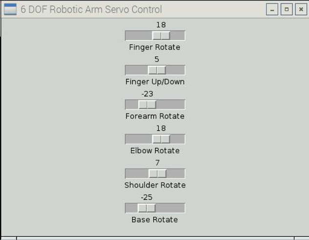
Figure 9-28 is a screenshot of the GUI showing the six labeled slider controls.
Figure 9-28 6-DOF_Robot_Arm program GUI.
I tested all the servos on the arm by moving the slider controls starting from the top to the bottom. The corresponding servo should move throughout its total range of motion. Just be careful to slowly move each slider because there is some mass to the arm, which, in turn, can create a significant force on the arm’s structure if moved rapidly. Remember that Newton’s second law, F = MA , still applies, and moving the slider rapidly creates a large acceleration A .
It is time to explore an interesting application for this 6-DOF robotic arm once you are satisfied that the arm operates as expected. Because the arm does not have a gripper, I decided to pursue a generalized Cartesian Coordinate positioning application based on the concept discussed earlier in this chapter. Please review the very brief section “X-Y-Z Coordinate (Cartesian Coordinate)” to refresh your memory before proceeding to the next section.
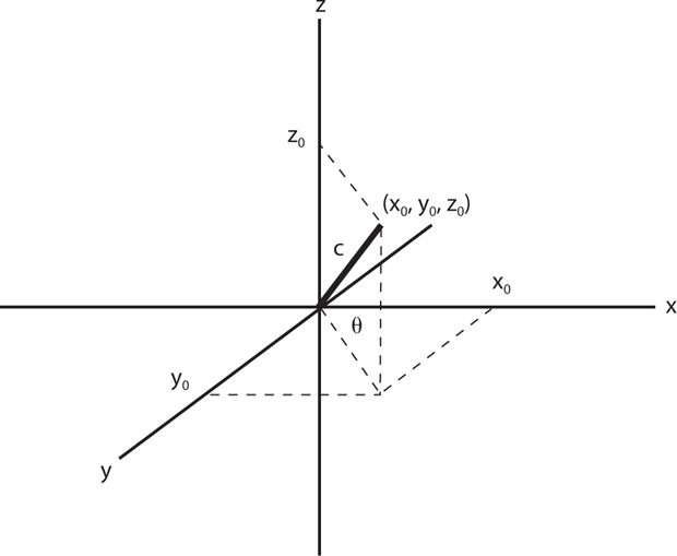
First, be forewarned that there is a bit of math in this section. However, it mostly concerns trigonometric functions, which I assume most of my readers (except for the younger ones) have been exposed to at some point in their educational experience. The primary purpose of this X-Y-Z Coordinate application (referred to from this point on as the app ) is to translate a given coordinate located in the 6-DOF arm’s volumetric workspace into servo angle commands for the base, shoulder, and elbow joints. You will see that just changing these three joint angles will position the fingers at any point in the volume corresponding to the given x , y , and z coordinates. Figure 9-29 is a vector diagram illustrating this configuration.
Figure 9-29 Vector diagram.
The given coordinate is shown in the diagram as a point located at x 0 , y 0 , and z 0 , which are points on the respective x , y , and z axes. The vector from the point of origin (0, 0, 0) is labeled c, and its length is determined by this formula:
c 2 = x 02 + y 02 + z 02
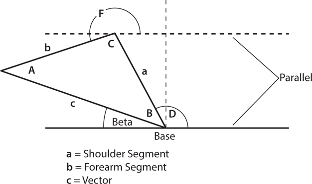
The angle θ shown on the diagram is the angle of the vector c projected onto the x-y plane and the x axis. This angle would be used to rotate the base such that the robotic arm points precisely in the direction of the given coordinate point. Determining the angles for both the shoulder and elbow joints is more complex but still doable. Figure 9-30 is a simplified diagram representing both the shoulder and forearm segments. The shoulder segment is labeled a and the forearm b .
Figure 9-30 Free-body diagram showing the shoulder, forearm, and vector segments.
I used the law of cosines to compute the angles A , B , and C shown in Figure 9-30 . The basic formula is
c 2 = a 2 + b 2 − 2 × a × b × cos(C )
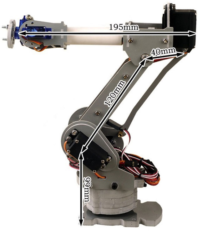
The values of segments a and b came from a SainSmart website diagram, shown in Figure 9-31 . The shoulder segment is 12 cm, and the forearm segment is 15.5 cm.
Figure 9-31 Segment lengths for a and b.
This next equation computes the C angle, which is part of an elbow joint servo angle:
cos(C ) = (a 2 + b 2 − c 2 )/(2 × a × b )
I used this next formula to compute the B angle, which is part of the shoulder joint:
cos(B ) = (a 2 − b 2 + c 2 )/(2 × a × c )
Of course, all the angle computations are done in radians and must be converted back into degrees using the relationship that 2π radians is equivalent to 360°.
There is one more angle that must be accounted for, and this is the angle β between the vector and the x-y plane. Looking at Figure 9-30 , it is straightforward to determine that this angle is computed as follows:
sin–1 (β) = z 0 /c
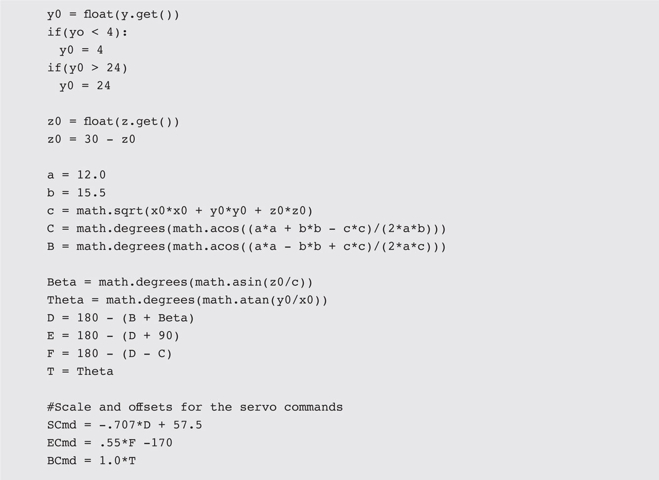
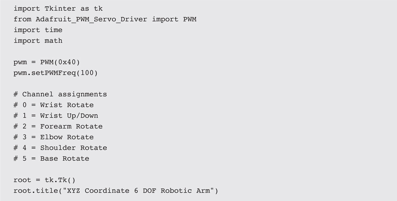
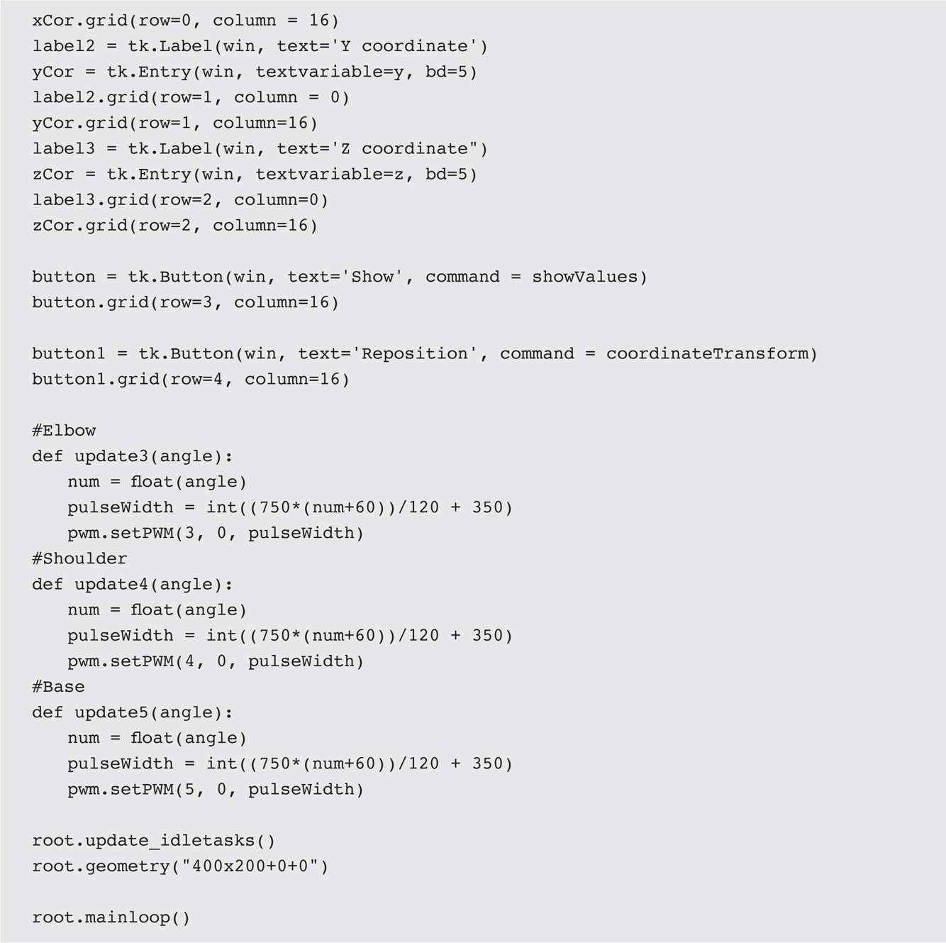
I incorporated all the mathematics I just went through into a function named coordinateTransform()
and added it to the 6-DOF_Robot_Arm.py program. I then rewrote 6-DOF_Robot_Arm.py to query the user for the x
, y
, and z
coordinates in centimeters. I also removed all the sliders because the purpose of this new app is to implement arm positioning based on coordinate inputs.
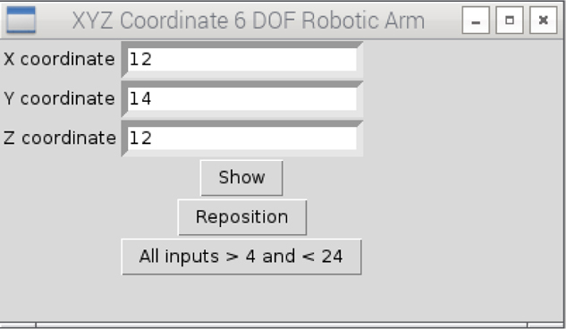
Once the x , y , and z coordinates are input, you will need to press the Reposition button to cause the arm to move. I did this as a safety feature because the robot will quickly reposition itself to the desired coordinate position in its workspace. I also limited the coordinate entries to be within the range of 4 to 24 cm such that the servos would stop moving before reaching their mechanical limits.
CAUTION
Be very careful because the robotic arm will swing quite rapidly if you enter new coordinates that are widely separated from its resting position. Keep small children, pets, and limbs away from the robotic arm while you run this program.
The changed program 6-DOF_Robot_Arm.py was renamed XYZ_Robot_Arm.py and is available on this book’s website and also listed next:


You should run the program in the same directory as all the other arm control programs. Enter the following to run this program:
![]()
Figure 9-32 is a screenshot of the program running with a set of x , y , and z coordinates entered. The arm started to reposition immediately after I clicked the Reposition button.
Figure 9-32 Screenshot of the XYZ_Robot_Arm program running.
You also may notice that I had the debugging print statements displayed because they helped me immensely to correctly modify the program such that it functioned as I wanted it to. I also included 1-second delays so that the individual segment positioning could be observed separately. You can easily remove them if you want all the segments and base to move together.
Before concluding this section, I want to mention some constraints and limitations within this program. The arm positioning can only be approximated because the point of origin I used in the geometric calculations differs from the real robotic arm. By this, I mean that the pivot where the shoulder segment rotates at the base is displaced approximately 4.5 cm from the vertical base rotation axis. This displacement will cause a constant error in the resulting angle calculations owing to the z -axis offset. I chose to leave the error in place because the robotic arm was designed for an educational/fun experience and not for a precision setup. There is also another slight deviation in that there is a small offset between the shoulder and elbow pivot points, again introducing some error in the angle calculations. Readers are encouraged to modify the program to reduce or eliminate these errors or simply use the program as is.
I have listed below several improvements and enhancements to this program that interested readers may explore further:
1. Incorporate a file I/O operation where a series of coordinates may be read in and the robotic arm would be continuously repositioned in accordance with the coordinates stored in the file.
2. Attach a felt-tipped pen to the end effector (fingers), and draw text and figures on a white sheet using only x and y coordinates to move the effector.
3. Attach a video camera to the end effector and feed the video stream to an image-processing program capable of recognizing simple objects, such as a ball or block. These programs usually have center-of-gravity capture algorithm that can provide control signals to the robotic arm to keep the observed object centered in the frame of the video stream.
Presenting these enhancements and improvements to the 6-DOF robotic arm concludes this section and the chapter.
The chapter began with a comprehensive introduction to robotic arms that explained the concepts and methodologies used in designing these devices. Two robotic arms were next introduced, and they were used as demonstrators to show how robotic arms actually function.
I next discussed how servos function as they are key components of all robotic arms. Software was discussed next, and I showed you how to configure a RasPi to control a robotic arm using the I2C bus. I also went through an initial test using a stand-alone servo to test the software installation and configuration process.
I next demonstrated a relatively simple 3-DOF arm used in a pick-and-place application that was programmed using Python. A 6-DOF arm was used next to demonstrate how a much more complex robotic arm worked. I wrote two Python programs to control this arm. The first simply allowed you to control each of the six servos using a GUI widget. The second program allowed you to enter x , y , and z coordinates and have the robotic arm reposition its end effector to the corresponding point in its volumetric workspace.
The chapter concluded with my presenting a few recommendations for future enhancements and improvements to the 6-DOF robotic arm.