Chapter 12
Climate Change and Human Health
Jonathan A. Patz and Howard Frumkin
Dr. Patz reports no conflicts of interest related to the authorship of this chapter. Dr. Frumkin's disclosures appear in the front of this book, in the section titled “Potential Conflicts of Interest in Environmental Health: From Global to Local.”
Climate change, whether resulting from natural variability or from human activity, depends on the overall energy budget of the planet, the balance between incoming (solar) shortwave radiation and outgoing longwave radiation. This balance is affected by the Earth's atmosphere, in much the same way that the glass of a greenhouse or a car's windshield on a hot day allows sunlight to enter and then traps heat (infrared) energy inside. An atmosphere with higher levels of so-called greenhouse gases will retain more of this heat and will result in higher average surface temperatures than will an atmosphere with lower levels of these gases.
A major source of information on climate change is the work of the United Nations Intergovernmental Panel on Climate Change (IPCC), which was established by the World Meteorological Organization (WMO) and the United Nations Environment Programme (UNEP) in 1988. Approximately every five years since 1990, most recently in 2014, the IPCC has conducted assessments of current scientific work on climate change, the potential impacts of this change, and various prevention options. Several national assessments have also been conducted; the third and most recent U.S. National Climate Assessment was published in 2014.
Greenhouse Gases
The composition of the Earth's atmosphere has changed since preindustrial times. These changes, which began around the mid-1700s, include increases in the atmospheric levels of carbon dioxide (CO2), methane (CH4), and nitrous oxide (N2O) that far exceed any changes occurring in the preceding 10,000 years. Historical levels of these gases are known from analyses of air trapped in bubbles in Antarctic ice cores. For example, the concentration of CO2 has risen by approximately 35%, from about 280 parts per million by volume (ppmv) in the late eighteenth century to about 400 ppmv at present.
These gases are known as greenhouse gases. They contribute to warming of the Earth—an effect called positive radiative forcing—by absorbing and then re-emitting infrared radiation toward the lower atmosphere and the Earth's surface. (Figure 12.1 summarizes the principal components of radiative forcing, and Table 12.1 shows today's concentrations of these greenhouse gases.)

Figure 12.1 Components of Radiative Forcing
Source: IPCC, 2013.
This figure shows the extent to which various factors—levels of certain gases, changes in land use, and so on—contribute to radiative forcing (as of 2005, relative to the start of the industrial era, in about 1750). Most of these factors result from human activity; the only exception was a natural increase in solar irradiance. Positive forcings lead to warming of the climate and negative forcings (principally aerosol particles that reflect and absorb solar energy and alter cloud properties) lead to cooling. The black line over each bar represents the range of uncertainty for the respective value.
Table 12.1 The Main Greenhouse Gases
| Greenhouse gases | Chemical formula | Preindustrial concentration (ppbv) | Concentration in 2012–2013 (ppbv) | Atmospheric lifetime (years) | Anthropogenic sources | Global warming potential (GWP)a |
| Carbon dioxide | CO2 | 278,000 | 395,000 | Variableb | Fossil fuel combustion, land use changes, cement production | 1 |
| Methane | CH4 | 700 | 11,762–1,893 | 12.2 ± 3 | Fossil fuel combustion, rice paddies, waste dumps, livestock | 21c |
| Nitrous oxide | N2O | 275 | 325 | 120 | Fertilizer, combustion, industrial processes | 310 |
| CFC-12 | CCl2F2 | 0 | 0.527 | 102 | Liquid coolants, foams | 6,200–7,100d |
| HCFC-22 | CHClF2 | 0 | 0.210–231 | 12.1 | Liquid coolants | 1,300–1,400d |
| Sulfur hexafluoride | SF6 | 0 | 0.007 | 3,20 | Dielectric fluid | 23,900 |
Note: ppbv = parts per billion by volume; CFC-12 = dichlorodifluoromethane; HCFC-22 = chlorodifluoromethane (both are used as refrigerants).
a GWP for 100-year time horizon.
b No single lifetime for CO2 can be defined because different sink processes have different rates of uptake.
c Includes indirect effects of tropospheric ozone water vapor production.
d Net global warming potential (i.e., including the indirect effect due to ozone depletion).
Sources: Carbon Dioxide Information Analysis Center, 2014.
A Warming Earth: From Past to Future
Long-term climate change, whether from natural sources or from human activity, can be observed as a signal against a background of natural climate variability. To help detect the meaning of this signal, we need to estimate natural variability using historical climate data. Because instrument records are available only for the recent past (a period of less than 150 years), previous climates must be deduced from paleoclimatic records, including tree rings, pollen series, faunal and floral abundances in deep-sea cores, isotope analyses of coral and ice cores, and for the more recent historical period, diaries and other documentary evidence. Results of these analyses show that surface temperatures in the mid- to late twentieth century appear to have been warmer than they were during any similar period in the last 600 years in most regions and in at least some regions warmer than in any other century for several thousand years.
About half of the anthropogenic greenhouse gas (GHG) emissions that occurred between 1750 and 2010 occurred after 1970. Growth in emissions has been greatest in the first decade of the twenty-first century (2.2% per year, compared with 1.3% from 1970 to 2000). Emissions continue to increase; 2011 emissions exceeded those in 2005 by 43% (IPCC, 2013), although 2014 may have marked a plateau. CO2 from fossil fuels and industrial processes accounted for ≈ 78% of the total increase from 1970 to 2010. Economic and population growth contribute most to increases in emissions globally and have outpaced improvements in energy efficiency.
Earth System Changes
Although the average effect across the Earth's surface is a warming, changing temperatures tell only part of the story. Higher temperatures evaporate soil moisture more quickly (contributing to severe droughts), but warm air can also hold more moisture than cool air, resulting in heavy precipitation events; such hydrological extremes (floods and droughts) are very much a part of climate change scenarios and of substantial concern to public health professionals. Additionally, the Arctic and Antarctic ice caps are melting, releasing vast amounts of water into the oceans, raising ocean levels, and potentially altering the flow of ocean currents. The weather patterns that result from these and other changes vary greatly from place to place and over short periods of time, emphasizing the importance of climate variability. For these reasons the term climate change is more accurate than global warming and is the accepted term for this set of changes.
Accordingly, the accelerating temperature changes noted earlier have been associated with corresponding Earth system changes. Since 1961, sea levels have risen on average by approximately 2 millimeters per year, and snow cover and glaciers have diminished in both hemispheres. Most striking is the extent to which the Arctic ice cap has melted in the past thirty years—by about 7.4% per decade (Figure 12.2). These trends are expected to continue. According to the IPCC, over the course of the twenty-first century, sea levels will rise between 26 and 98 centimeters, and floods and droughts will continue to intensify.
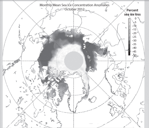
Figure 12.2 The Melting of Arctic Sea Ice
Adapted from: National Snow & Ice Data Center, 2015.
This map—a view from above the North Pole—shows the extent of Arctic sea ice in October 2012 compared with the average over the preceding three decades. It shows a dramatic decrease in sea ice concentration, the fraction of the ocean covered by sea ice. (The grey circle centered over the North Pole indicates where the central Arctic is not visible to the satellite instruments used to generate these maps.) The loss of arctic sea ice is an example of a feedback loop. During the summer months, sea ice can reflect as much as 70% of incoming solar radiation back to space. When sea ice disappears, the dark ocean surface absorbs much of the incoming radiation, reflecting less than 10%. This extra energy increases the ocean temperature and the temperature of the overlying atmosphere, contributing further to global warming.
Ocean Temperatures and Hurricanes
Records indicate that sea surface temperatures have increased steadily over the last one hundred years, and more sharply over the last thirty-five years. Recent decades have repeatedly set records for sea surface temperatures, with 2014 the warmest year on record (www.ncdc.noaa.gov/sotc/global).
Uncertainty exists over whether hurricane frequency will increase, but evidence points to more extreme hurricanes (categories 4 and 5) (Bender et al., 2010; IPCC, 2013). Sea level rise will continue to exacerbate storm surges, worsen coastal erosion, and inundate low-lying areas. Salinization of aquifers likely will augment challenges to coastal cities and towns.
Sea Level Rise
Sea level has risen approximately 20 cm over the last 100 years, far more than in the two previous millennia, an increase associated with thermal expansion of sea water and with melting glaciers. While sea level is likely to rise between 26 and 98 cm by 2100, more extreme estimates that envision catastrophic melting events reach as high as >200 cm. (This is called a tail risk—the extreme end of the distribution of probabilities for a particular outcome.)
One expected effect of sea level rise is an increase in flooding and coastal erosion in low-lying coastal areas. This will endanger large numbers of people; fourteen of the world's nineteen current megacities are situated at sea level. Coastal regions at risk of storm surges will expand and the population at risk will increase from the current 75 million to 200 million (McCarthy, Canziani, Leary, Dokken, & White, 2001). For Bangladesh, a 1.5 meter rise is projected to have even more catastrophic consequences. Countries such as Egypt, Vietnam, Bangladesh, and small island nations are especially vulnerable, for several reasons. Coastal Egypt is already subsiding due to extensive groundwater withdrawal, and Vietnam and Bangladesh have heavily populated, low-lying deltas along their coasts.
Rising sea levels may affect human health and well-being indirectly, in addition to direct effects through inundation or heightened storm surges. Rising seas, in concert with withdrawal of freshwater from coastal aquifers, could result in saltwater intruding into those aquifers and could also disrupt stormwater drainage and sewage disposal.
Particularly Vulnerable Regions
Certain regions and populations are more vulnerable than others to the health impacts of climate change (Hess, Malilay, & Parkinson, 2008). These vulnerable areas include
- Areas or populations within or bordering regions with a high endemicity of climate-sensitive diseases (such as malaria)
- Areas with an observed association between epidemic disease and weather extremes (e.g., El Niño–linked epidemics)
- Areas at risk from combined climate impacts relevant to health (e.g., stress on food and water supplies or risk of coastal flooding)
- Areas at risk from concurrent environmental or socioeconomic stresses (e.g., local stresses from land-use practices or an impoverished or undeveloped health infrastructure) and with little capacity to adapt
These Earth system changes have complex direct and indirect implications for human health, as illustrated in Figure 12.3. This figure, crafted by Dr. Tony McMichael, a seminal thinker regarding the health impacts of global change, reflects the ecological approach presented in Chapter 2. It depicts the interacting physical, social, and economic processes that determine health. The following sections of this chapter address major categories of anticipated health effects of climate change. These include malnutrition (possibly the largest problem); risks from weather extremes and disasters such as heat and cold, storms and flooding, and drought and wildfires; air pollution and aeroallergens; infectious diseases, including those that are waterborne, foodborne, and vector-borne; mental health effects; and the effects of armed conflict and dislocation. The last section of the chapter addresses the public health response to climate change, from preparedness to greenhouse gas mitigation. Co-benefits of mitigation are considered, as well as the ethical dimensions of climate change and health.
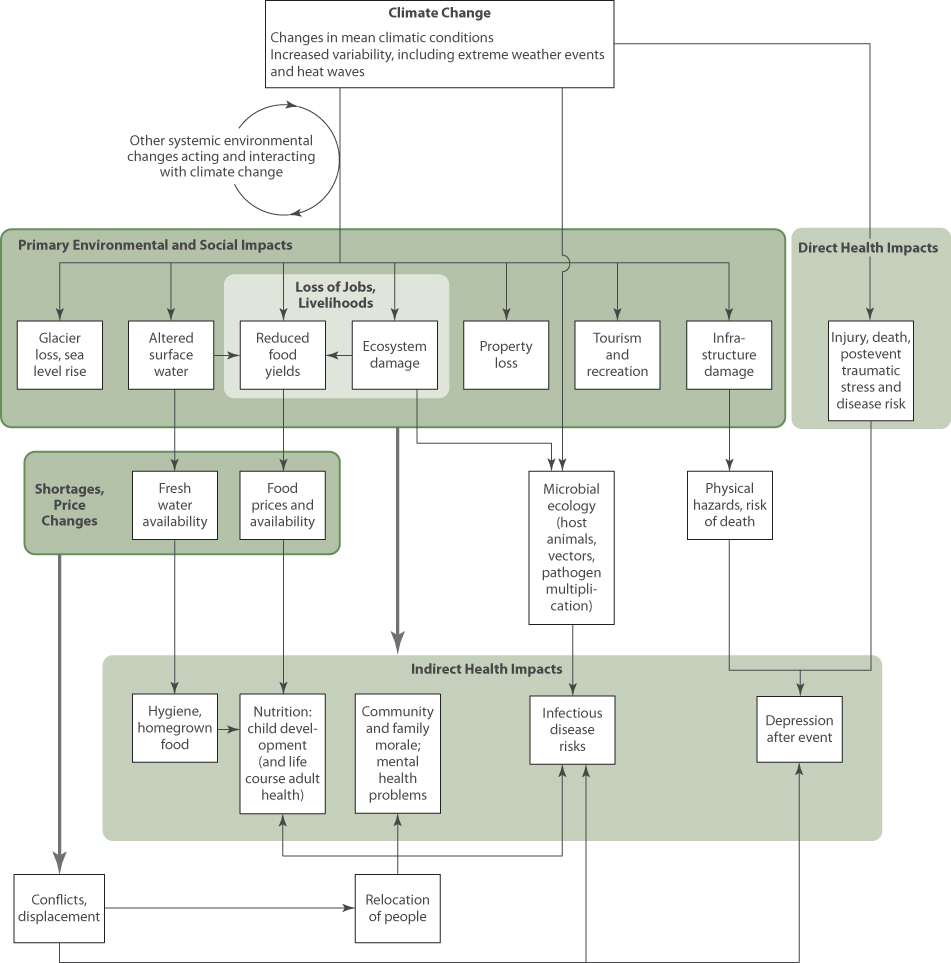
Figure 12.3 Processes and Pathways Through Which Climate Change Influences Human Health
Source: McMichael, 2013.
Food and Malnutrition
Malnutrition is one of the most pressing health concerns in the context of the changing climate. Three mechanisms affect food security: reduced crop yields, increased crop losses, and decreased nutrient content.
On average, climate change is projected to reduce global food production by up to 2% per decade, even as demand increases by 14% (Porter et al., 2014). More than 800 million people currently experience chronic hunger, concentrated in areas where productivity could likely be most affected (Food and Agriculture Organization of the United Nations [FAO], 2013; Wheeler & von Braun, 2013). Major contributors to reduced yields will be water shortages (especially for glacial melt–dependent regions in Asia, Europe, and South America) and hotter temperatures (because most cultivars are already growing close to their thermal optimum). Wheat, maize, sorghum, and millet yields are estimated to decline by approximately 8% across Africa and South Asia by 2050 (Porter et al., 2014). By 2050, around 25 million more children might be undernourished as the result of climate change, and rates of growth stunting could increase substantially (Nelson et al., 2009; Lloyd, Sari Kovats, & Chalabi, 2011). Climate change-related price shocks (rapid rises in food prices), especially for staples such as corn and rice, could more than double by mid-century, placing impoverished populations at further risk (Bailey, 2011).
Plant diseases caused by fungi, bacteria, viruses, and oomycetes, already responsible for a 16% global crop loss, may substantially increase with climate change (Chakraborty & Newton, 2011). In addition, climate change favors the growth of many weeds, which compete with crops (Ziska & McConnell, 2015). Also, the nutrient value of some crops may diminish. CO2 “fertilization” can reduce the protein content in wheat and rice, and the iron and zinc content in crops such as rice, soybeans, wheat, and peas (S. S. Myers et al., 2014).
Adaptive measures range from drought- or salt-resistant crops to improved technology such as drip irrigation and hoop houses (inexpensive greenhouses). Other potential adaptation strategies include changing planting dates, increasing crop diversity, reducing waste, increasing cropping efficiency, and changing diets.
An indirect pathway by which climate change may affect crops is biofuel production. Some crops and cropland will be diverted from food to fuel. While the impacts are controversial, this diversion may have unintended consequences, contributing to food shortfalls and rising food prices (Tirado, Cohen, Aberman, Meerman, & Thompson, 2010; Harvey & Pilgrim, 2011; HLPE, 2013).
In addition to reducing crop production, climate change will affect food availability in another way: through its effects on fisheries and aquaculture. According to the FAO (2013), 540 million people globally depend on wild fisheries and aquaculture as sources of protein and income. For the poorest 80% of these, fish represents at least half of their animal protein and dietary minerals. Climate change will affect river and marine ecosystems and threaten fish availability, through many pathways. A key issue is ocean acidification; oceans have absorbed about 30% of anthropogenic CO2, their surface pH has become 0.1 units more acidic since the beginning of the industrial era, and IPCC scenarios predict a further drop in global surface ocean pH of between 0.14 and 0.35 units over the twenty-first century (IPCC, 2013). Ocean acidification threatens marine shell-forming organisms (such as corals) and their dependent species. Other challenges to fisheries include altered river flows, destructive coastal storms, and the spread of pathogens (Cochrane, De Young, Soto, & Bahri, 2009; Porter et al., 2014).
Weather Extremes and Disasters
Extreme temperatures, severe storms, rising sea levels, and floods, droughts, and wildfires are all threats to public health. Although slight changes in the average blood pressure or cholesterol level across a population can represent a health risk, in the case of climate it is the extremes of temperature and in the water cycle that threaten human health.
Heat Waves
Extremes of both hot and cold temperatures are associated with higher morbidity and mortality compared to the intermediate, or comfortable, temperature range (Kilbourne, 2008). The relationship between temperature and morbidity and mortality is J-shaped, with a steeper slope at higher temperatures.
The body's thermoregulatory mechanisms can cope with a certain amount of temperature rise through control of perspiration and vasodilation of cutaneous vessels. The ability to respond to heat stress is thus limited by the capacity to increase cardiac output as required for greater cutaneous blood flow. Over time, people can adapt to high temperatures by increasing their ability to dissipate heat through these mechanisms. Heat-related illnesses range from heat exhaustion to kidney stones (which increase with dehydration).
Epidemiologists quantify heat-related mortality in two ways: tabulating death certificates that cite heat as a cause, and tracking mortality increases across populations during heat waves—periods of unusually hot weather, defined by the World Meteorological Organization as more than five consecutive days with temperatures at least 5°C above the average maximum temperature during the 1961 to 1990 baseline period. The first approach typically leads to underestimates, because heat-related deaths are routinely attributed to cardiovascular and other causes without citing heat as the underlying factor. In the United States, an average of 658 deaths are certified as heat-related each year, representing more fatalities than all other weather events combined (Luber & McGeehin, 2008; Centers for Disease Control and Prevention [CDC], 2013). More accurate risk estimates compare observed versus expected mortality during heat events; for example, 70,000 excess deaths were estimated for the 2003 European heat wave and 15,000 for the 2010 Russian heat wave (Robine et al., 2008; Matsueda, 2011).
Heat waves have been growing more frequent, more intense, and longer in duration over recent decades (Habeeb, Vargo, & Stone, 2015), and this trend is expected to continue, especially in the high latitudes of North America and Europe (Goodess, 2013). “Mega” heat waves (as have occurred in Europe and Russia) are projected to increase in frequency by five- to tenfold within the next forty years (Barriopedro, Fischer, Luterbacher, Trigo, & García-Herrera, 2011). Figure 12.4 shows the projected number of extremely hot days each year in Milwaukee, Atlanta, New York City, and Dallas (defined as above 32°C [90°F] in the first three cities, and above 38°C [100°F] in Dallas). Each city will confront a marked increase in hot days—for example, a tripling in New York (Patz, Frumkin, Holloway, Vimont, & Haines, 2014). These trends will have serious public health consequences. While air conditioning and preparedness have reduced heat-related deaths and illness in the United States (Kalkstein, Greene, Mills, & Samenow, 2011), climatic and demographic trends (such as the aging population) suggest that risks may persist. One estimate, focusing on a set of twelve U.S. cities, projected over 200,000 excess heat-related deaths during the twenty-first century (Petkova et al., 2014). While the reduction of extremely cold days will avoid some cold-related deaths, this reduction is not expected to balance the increase in heat-related deaths (Luber et al., 2014).
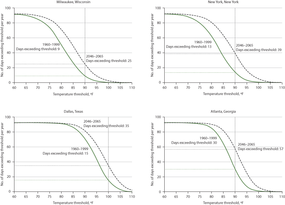
Figure 12.4 Number of Days in June, July, and August When Daytime Maximum Temperatures Exceed a Given Threshold (indicated by a vertical line)
Source: Patz et al., 2014.
The solid-line curves show observations from 1960–1999, and the dotted-line curves, shifted to the right, show projected distributions for 2046–2065 under a business-as -usual emissions scenario. A relatively small shift can lead to a substantial change in the area under the steep portion of the curve.
The epidemiology of heat waves has been well studied, and vulnerability and protection factors are well known. People who are most vulnerable include the poor, the elderly, those who are socially isolated, those who lack air conditioning, and those with certain medical conditions that impair the ability to dissipate heat. A particular risk factor is living in cities, especially in hot parts of cities, because of the heat island effect.
An urban heat island is an urban area that generates and retains heat as a result of buildings, human and industrial activities, and other factors (Figure 12.5). Black asphalt and other dark surfaces (on roads, parking lots, and roofs) have a low albedo (reflectivity); they absorb and retain heat, reradiating it at night, when the area would otherwise cool down. In addition, urban areas are relatively lacking in trees, so they lose the cooling effect associated with evapotranspiration.
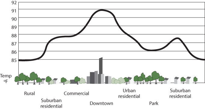
Figure 12.5 Urban Heat Island Profile
Source: WikiMedia Commons, 2011.
The urban heat island results from dark surfaces, loss of tree canopy, and concentrated generation of heat. Some neighborhoods in a city are far warmer than others, due to local factors such as topography and building types.
An interesting aspect of heat, and one with both health and economic consequences, is its impact on people at work. Outdoor workers such as farmworkers and construction workers, and those in facilities without air conditioning, such as garment factories in poor nations, are most directly affected by heat. The reduction in their work capacity can be substantial, with serious economic consequences. One study estimates that ambient heat stress has reduced global labor capacity by 10% at summer's peak over the past few decades (Dunne, Stouffer, & John, 2013), and by mid-century, workdays lost due to heat could reach 15% to 18% in Southeast Asia, West and Central Africa, and Central America (Kjellstrom, Holmer, & Lemke, 2009). These regions contain some fragile economies, which could be particularly susceptible to reduced labor capacity.
Climate-Related Disasters
Floods, droughts, and extreme storms have claimed millions of lives during recent years and have adversely affected the lives of many more millions of people and caused billions of dollars in property damage. According to the International Federation of Red Cross and Red Crescent Societies (IFRC), an average of 114,992 people died each year due to natural disasters during the period from 2003 to 2012 (Vinck, 2013). (The IFRC's World Disasters Report draws from the EM-DAT International Disaster Database at the Centre for Research on the Epidemiology of Disasters [CRED] at the University of Louvain, which is cited extensively in Chapter 24.) The number of people affected by natural disasters is two orders of magnitude greater than the number killed (CRED, 2015). In addition to causing acute deaths and injuries, disruption of health care, and lasting health impacts such as mental health disorders, disasters can halt or reverse economic growth and profoundly disrupt social structures.
Floods and Heavy Rain
Floods are the most common type of natural disaster worldwide, with between 150 and 200 major floods occurring annually (Vinck, 2013). Increased severe rainstorms are one contributor. In the United States, the amount of precipitation falling in the heaviest 1% of rain events increased by 20% during the past century, and total precipitation increased by 7%. Over the last century the upper Midwest experienced a 50% increase in the frequency of days with precipitation of over four inches (Kunkel, Easterling, Redmond, & Hubbard, 2003). Other regions, notably the South, have also seen marked increases in heavy downpours, with most of these events coming in the warm season and almost all of the increase coming in the last few decades.
Heavy rains can increase the risk of waterborne diseases, a risk discussed below in the section on infectious diseases. They can also result in flooding that kills, injures, and displaces people. Population concentrations in high-risk areas such as floodplains and coastal zones increase vulnerability to floods. Degradation of the local environment can also contribute significantly to vulnerability. For example, Hurricane Mitch, the most deadly hurricane to strike the Western Hemisphere in the last two centuries, caused 11,000 deaths in Central America, with thousands more people recorded as missing. Many fatalities occurred during mudslides in deforested areas (National Climatic Data Center, 1999).
Wildfires
The incidence of extensive wildfires (those burning over 400 hectares each) in the Western United States rose fourfold between the period from 1970 to 1986 and the period from 1987 to 2003 (Westerling, Hidalgo, Cayan, & Swetnam, 2006). Several climate-related factors may have played a role in this increase: droughts that dried out forests; higher springtime temperatures that hastened spring snowmelt and thereby lowered soil moisture; and the rise of some tree pest species (Running, 2006; Westerling et al., 2006). Forecasts call for an increased risk of wildfires in many (but not all) areas over the course of the twenty-first century (Moritz et al., 2012).
Wildfires threaten health both directly and through reduced air quality. Fire smoke carries a large amount of fine particulate matter that exacerbates cardiac and respiratory problems such as asthma and chronic obstructive pulmonary disease (COPD). A study on worldwide mortality estimated 339,000 premature deaths per year (with a possible range of 260,000–600,000 deaths) attributable to pollution from forest fires, especially particulates (Johnston et al., 2012).
Air Pollution
Climate change may affect exposure to air pollutants in many ways because it can influence both the levels of pollutants that are formed and the ways in which these pollutants are dispersed. Air quality is likely to suffer with a warmer, more variable climate (Bernard, Samet, Grambsch, Ebi, & Romieu, 2001).
Ozone
Ozone is an example of a pollutant whose concentration may increase with a warmer climate. As explained in Chapter 13, higher temperatures increase ozone formation from precursors—a relationship demonstrated in many cities, and shown graphically in Figure 12.6. Accordingly, the ozone season in affected cities occurs during the summer, when warmer temperatures promote ozone formation. (Particulate matter formation can also increase at higher temperatures, due to increased gas-phase reaction rates.) This suggests that hotter summers will worsen air quality. However, air pollution chemistry is complex, and other factors—from changing vegetation to policies that reduce methane emissions—will also play a role, leading to variability from place to place (Fiore, Naik, & Leibensperger, 2015).

Figure 12.6 The Relationship Between Temperature and Ozone Levels in Santiago, Chile
Source: Rubio & Lissi, 2014.
This graph shows the association between measured maximum temperature, and the average eight-hour ozone level, measured in Santiago's O'Higgins Park. In studies in cities around the world, hot days feature higher ozone levels.
The role of vegetation is especially interesting. As explained in Chapter 13, many species of trees emit volatile organic compounds (VOCs) such as isoprenes, which are precursors of ozone. Isoprene production is highly responsive to leaf temperature and light. Under the right circumstances, higher levels of isoprenes result in higher levels of ozone (Squire et al., 2015).
The relationship between climate change and air pollution is complex. Many feedback loops operate, some helpful and others harmful. On the one hand, some particles in the air reflect radiant energy and can help to cool the atmosphere; the best-known example is the cooling that follows major volcanic eruptions. On the other hand, a warmer climate will mean more demand for energy to power air conditioners, resulting in more air pollution (if fossil fuel plants supply the power). Overall, for air pollution, as for many other aspects of climate change, the impacts are not fully understood, but potential threats to public health deserve careful attention.
Aeroallergens
Pollen is another air contaminant that may increase with climate change. Higher levels of carbon dioxide promote growth and reproduction by some plants, including many that produce allergens. Ragweed plants experimentally exposed to high levels of carbon dioxide can increase their pollen production several-fold. Over half the U.S. population (55%) tests positive for allergens, and over 34 million have asthma (Allergy USA, 2014). In recent decades the allergy season has lengthened with earlier flowering of some species, such as oaks, and levels of allergens such as ragweed (Ambrosia) pollen have risen, a predictable effect of higher temperatures and CO2 levels (Zhang et al., 2015). Ragweed season has been lengthening since the mid-1990s, particularly at higher latitudes along a 1,600-mile north-south sampling of monitoring stations through mid-North America (Ziska et al., 2011).
Aeroallergens are not the only allergens to become more troublesome with climate change. With higher levels of carbon dioxide, poison ivy grows more exuberantly, and its allergen, urushiol, becomes more allergenic. Unhappily, poison ivy seems to enjoy a special advantage compared to other plants; its vines grow twice as much per year in air with doubled preindustrial carbon dioxide levels as in unaltered air, a fivefold greater increase than reported for other plant species (Mohan et al., 2006). Emerging evidence suggests that other allergenic species respond to climate change by becoming more harmful; researchers have observed enhanced growth of weeds such as stinging nettle and leafy spurge, which cause rashes following skin contact (Ziska, 2003), greater allergenicity of Aspergillus (Lang-Yona et al., 2013), and extended ranges and active seasons for some stinging insects.
Infectious Diseases
A range of infectious diseases can be influenced by climate conditions. The diseases most sensitive to influence by ambient climate conditions are those spread not by person-to-person pathways but directly from the source: the waterborne and foodborne diseases as well as vector-borne diseases (which involve insects and/or rodents in the pathogen's life cycle). For each of these infectious diseases, climate factors interact with a range of other factors: land-use patterns (deforestation, road construction, urbanization, dam construction), disease control programs, and others. Accordingly, these diseases, and the ways in which climate change affects them, are best considered through the lens of ecological thinking (see Chapter 2).
Waterborne Diseases
Waterborne diseases are likely to become a greater problem as climate change continues and affects both freshwater and marine ecosystems. In freshwater systems, both water quantity and water quality can be affected by climate change. In marine waters, changes in temperature, ph, and salinity will affect coastal ecosystems in ways that may increase the risk of certain diseases.
Freshwater Ecosystems
Waterborne diseases are particularly sensitive to changes in the hydrological cycle. Many community water systems are already overwhelmed by extreme rainfall events. Flooding can contaminate drinking water with runoff from sewage lines, containment lagoons (such as those used in animal feeding operations), or nonpoint source pollution (such as agricultural fields) across watersheds. Runoff can exceed the capacity of the sewer system or treatment plants, which then discharge the excess wastewater directly into surface water bodies. Urban watersheds sustain more than 60% of their annual contaminant loads during storm events (Fisher & Katz, 1988).
Thus it is no surprise that outbreaks of such diseases as cryptosporidiosis and giardiasis are associated with prior heavy rainstorms (Curriero, Patz, Rose, & Lele, 2001; Cann, Thomas, Salmon, Wyn-Jones, & Kay, 2013). Childhood gastrointestinal illness in the United States (Uejio et al., 2014) and India (Bush et al., 2014) has been linked to heavy rainfall. A Dutch study showed a 33% increase in gastrointestinal illness associated with sewage overflow following heavy rain; flood waters contained Campylobacter, Giardia, Cryptosporidium, noroviruses, and enteroviruses (De Man et al., 2014). An infamous example of heavy rain contributing to an outbreak was the 1993 Milwaukee cryptosporidiosis outbreak (Rose, 1997), which sickened over 400,000 and killed over 100.
With climate change projected to result in more severe and frequent precipitation events, the risk of waterborne diseases is expected to rise (Patz & Hahn, 2013). Using 2.5 inches (6.4 cm) of daily precipitation as the threshold for initiating a combined sewer overflow (CSO) event, the frequency of such events in Chicago is expected to rise by 50% to 120% by the end of this century (Patz Vavrus, Uejio, & McLellan, 2008), posing increased risks to drinking and recreational water quality.
Intense rainfall can also contaminate recreational waters and increase the risk of human illness (Schuster et al., 2005). For example, heavy runoff leads to higher bacterial counts in rivers in coastal areas and at coastal beaches, especially at the beaches near river outflows (Dwight, Semenza, Baker, & Olson, 2002). This suggests that the risk of swimming at some beaches increases with heavy rainfall, a predicted consequence of climate change.
Marine Ecosystems
Warm water and nutrient loading (primarily with nitrogen and phosphorus) favor blooms of marine algae, including two groups, dinoflagellates and diatoms, that can release toxins into the marine environment. These harmful algal blooms (HABs)—previously called red tides—can cause acute paralytic, diarrheic, and amnesic poisoning in humans, as well as extensive die-offs of fish, shellfish, and marine mammals and birds that depend on the marine food web. Over recent decades the frequency and global distribution of harmful algal blooms appear to have increased, along with more human intoxication from algal sources (Anderson, Cembella, & Hallegraeff, 2012). These have occurred both in marine settings and in freshwater lakes, such as Lake Erie (Figure 12.7). For example, in the summer of 2012, a group of seven vacationers on the Washington coast harvested mussels, prepared them in a soup, and ate them; within hours they experienced paresthesias, a “floating” sensation, nausea, vomiting, ataxia, and other symptoms. They were diagnosed with paralytic shellfish poisoning, a condition caused by eating fish or shellfish contaminated by saxitoxin, an algal product more toxic than sodium cyanide (Hurley, Wolterstorff, MacDonald, & Schultz, 2014). Of note, the number of cases reported in 2012 was substantially higher than in previous years; this was attributed to an unusually warm, sunny summer. Climate change is predicted to increase the frequency of such episodes, and in addition, ocean acidification may increase the toxicity of some algal species (Fu, Tatters, & Hutchins, 2012; Glibert et al., 2014). Ciguatera, a form of poisoning caused by ingesting fish that contains toxins from any of several dinoflagellate species, could also expand its range. This condition has been linked to sea surface temperatures, and as these warm, according to one projection, ciguatera fish poisoning could increase by two- to fourfold over the coming century (Gingold, Strickland, & Hess, 2014).
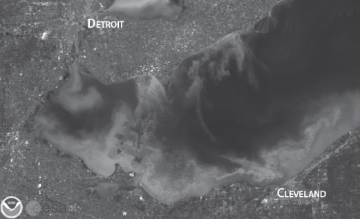
Figure 12.7 Satellite Photo of a Harmful Algal Bloom in Lake Erie in 2011
Source: National Oceanic and Atmospheric Administration, 2014.
This was the worst bloom in recent history, impacting over half the lake shore.
Some bacteria, especially Vibrio species, also proliferate in warm marine waters (Pascual, Rodó, Ellner, Colwell, & Bouma, 2000). Copepods (or zooplankton), which feed on algae, can serve as reservoirs for V. cholerae and other enteric pathogens. For example, in Bangladesh, cholera follows seasonal warming of sea surface temperatures, which can enhance plankton blooms (Colwell, 1996). Other Vibrio species have expanded in northern Atlantic waters in association with warm water (Thompson et al., 2004). For example, in 2004 an outbreak of V. parahaemolyticus shellfish poisoning was reported from Prince William Sound in Alaska. This pathogenic species of Vibrio had not been isolated from Alaskan shellfish previously due to the coldness of the Alaskan waters. What could have caused the species' expanded range? Water temperatures during in the 2004 shellfish harvest remained above 15°C, and mean water temperatures were significantly higher than they had been during the previous six years (McLaughlin et al., 2005). Such evidence suggests the potential for warming sea surface temperatures to increase the geographic range of shellfish poisoning and Vibrio infections into temperate and even arctic zones.
The incidence of diarrhea from other pathogens also shows temperature sensitivity, which may in turn signal sensitivity to changing climate. During the 1997 and 1998 El Niño event, winter temperatures in Lima, Peru, increased more than 5°C above normal, and the daily hospital admission rates for diarrhea more than doubled compared to rates over the prior five years (Checkley et al., 2000) (Figure 12.8)—a pattern that has been confirmed in multiple settings (Vezzulli, Colwell, & Pruzzo, 2013). Long-term studies of the El Niño–Southern Oscillation, or ENSO, have confirmed this pattern. ENSO refers to natural year-to-year variations in sea surface temperatures, surface air pressure, rainfall, and atmospheric circulation across the equatorial Pacific Ocean. This cycle provides a model for observing climate-related changes in many ecosystems. Sea surface temperature has had an increasing role in explaining cholera outbreaks in recent years (Vezzulli et al., 2013), as has ENSO, perhaps because of concurrent climate change (Rodó, Pascual, Fuchs, & Faruque, 2002). Overall there is growing evidence that climate change can contribute to the risk of waterborne diseases in both marine and freshwater ecosystems.

Figure 12.8 The Association Between Temperature and Childhood Diarrhea, Peru, 1993–1998
Source: Checkley et al., 2000.
Daily time series between January 1, 1993, and November 15, 1998, for admissions for diarrhea and for mean ambient temperature in Lima, Peru. Shaded area represents the 1997–1998 El Niño event.
Foodborne Diseases
More frequent warm days, greater humidity, and other climate-related factors can affect the persistence and dispersal of foodborne pathogens in many ways, and can increase the risk of foodborne infectious diseases (Hellberg & Chu, 2015). (As described in Chapter 16, waterborne and foodborne diseases can be hard to distinguish from each other, because contaminated water often contaminates food.) Data from many parts of the world show a strong association between temperature and the incidence of food poisoning with various pathogens—Campylobacter, Salmonella, Cryptosporidium, Shigella, and Giardia—showing different time lags between peak temperature and the peak in infections, and with the effect most pronounced at especially high temperatures (Kovats et al., 2004; Naumova et al., 2007). Not surprisingly, modeling suggests a sharp increase in foodborne illness with continued climate change. For example, one study, focusing on Beirut, projected a 16% to 28% increase by mid-century, and an increase of up to 42% by 2100 (El-Fadel, Ghanimeh, Maroun, & Alameddine, 2012). Improved food-handling practices, which play a major part in prevention, are therefore an important aspect of climate change adaptation (Lake et al., 2009).
Vector-Borne Diseases
Vector-borne diseases are infectious diseases, caused by protozoa, bacteria, and viruses, that are spread by organisms such as mosquitoes and ticks. The life cycle of these pathogens involves much time outside the human host and therefore much exposure to and influence by environmental conditions. The term tropical diseases is a reminder that each pathogen or vector species thrives in a limited range of climatic conditions.
The incubation time of a vector-borne infectious agent within its vector organism is typically very sensitive to changes in temperature and humidity (Patz et al., 2003). Many other mechanisms govern the impact of climate change on vector-borne diseases, as shown in Text Box 12.1 geographic shifts of vectors or reservoirs; changes in rates of development, survival, and reproduction of vectors, reservoirs, and pathogens; and increased biting by vectors and prevalence of infection in reservoirs or vectors (Medlock & Leach, 2015). All affect transmission to humans, such that exposure to vector-borne disease will likely worsen in a warmer world (Mills, Gage, & Khan, 2010; Patz & Hahn, 2013).
Mosquito-Borne Diseases
Malaria and arboviruses are transmitted to humans by mosquitoes. Because insects are cold-blooded, climate change can shift the distribution of mosquito populations, affect mosquito biting rates and survival, and shorten or lengthen pathogen development time inside the mosquito, factors that ultimately determine infectivity.
Malaria remains a scourge in many parts of the world. Despite considerable progress in fighting this disease in recent decades, it still accounts for over a million deaths each year, about 90% of these in Africa (Murray et al., 2012). Malaria risk is complex, and varies with demographic shifts, control measures, and other factors (Parham et al., 2015). However, malarial mosquito populations can be exquisitely sensitive to warming; an increase in temperature of just half a degree centigrade can translate into a 30% to 100% increase in mosquito abundance, an example of biological amplification by temperature effect (Pascual, Ahumada, Chaves, Rodó, & Bouma, 2006). Accordingly, most models forecast global increases in malaria risk over the next century, especially in highland regions of Africa, Asia, and Latin America (with some reduction of risk in tropical regions) (Caminade et al., 2014), emphasizing the importance of malaria control measures as a part of climate adaptation.
Arboviruses include the causative agents of dengue fever, West Nile virus, chikungunya, and Rift Valley fever. Dengue and chikungunya are transmitted by Aedes mosquitoes, West Nile virus by Culex mosquitoes, and Rift Valley fever usually through contact with the blood or organs of infected animals but also by Aedes mosquitoes. The four diseases differ clinically and epidemiologically, and have distinct geographic ranges. For example, Rift Valley fever has generally been confined to east Africa, although it has recently spread to other parts of Africa and to the Arabian peninsula, while dengue fever is widespread across south Asia, Africa, and Latin America. However, the four diseases also share important features, all relevant to climate change. First, there is evidence that climatic conditions, such as temperature and rainfall, can affect their spread. Second, the geographic range of all four diseases has expanded in recent decades. Third, modeling projects the potential for further spread with continued climate change. Finally, for each disease, infection reflects complex interplays of behavior, land use, mosquito control strategies, and other factors, so controlling these diseases in the face of climate change will be a complex challenge (Martin et al., 2008; Dhiman, Pahwa, Dhillon, & Dash, 2010; Weaver & Reisen, 2010; Morin et al., 2013; Campbell et al., 2015; Paz, 2015).
Tick-Borne Disease
Lyme disease is a tick-borne disease that was first described in the 1970s and has since become prevalent in North America, Europe, and Asia. The ecology and infectivity of this disease are related to many factors, such as habitat fragmentation and increased human contact with the mammals (deer, mice, and others) that carry the vector, the Ixodes tick. However, the tick life cycle is strongly influenced by temperature and other weather factors; for example, cold weather is limiting (Ostfeld & Brunner, 2015). The tick range has been expanding, and warming temperatures are projected to shift the range limit for this tick northward by 200 km by the 2020s and 1,000 km by the 2080s (Ogden et al., 2006).
Rodent-Borne Diseases
Rodent populations can be affected by weather, raising the potential for the diseases they transmit to be climate responsive. Examples of these diseases include hantavirus infection, leptospirosis, and plague.
Hantavirus infections are transmitted largely by exposure to infectious excreta from rodents and may cause serious disease and a high fatality rate in humans. Hantavirus pulmonary syndrome emerged in the southwestern United States in 1993, after an El Niño brought heavy rains, which in turn led to a growth in rodent populations (Glass et al., 2000). Leptospirosis, a bacterial disease that can feature pulmonary hemorrhage, meningitis, and kidney failure, is transmitted through the urine of infected rodents and other mammals. Events that increase exposure to rodents, such as extreme flooding, can greatly increase the risk of contracting this disease (Lau, Smythe, Craig, & Weinstein, 2010). Finally, plague is caused by the bacteria Yersinia pestis, which is transmitted by fleas, whose primary reservoir host is rodents. Plague also varies with weather and across seasons (Ben Ari et al., 2011). In fact, historical tree-ring data suggest that during the major plague epidemics of the Black Death period (1280 to 1350), climate conditions were becoming both warmer and wetter (Stenseth et al., 2006).
Mental Health Effects
Mental health disorders such as depression and anxiety cause major morbidity worldwide (Whiteford et al., 2013). Climate change may threaten mental health in several ways (Fritze, Blashki, Burke, & Wiseman, 2008; Berry, Bowen, & Kjellstrom, 2010; Doherty & Clayton, 2011).
Mental Health Impacts of Climate-Related Disasters
Following disasters such as floods and wildfires, mental health consequences such as post-traumatic stress, depression, and anxiety are common, and may represent a major part of the resulting health burden (North & Pfefferbaum, 2013; Goldmann & Galea, 2014). Several months after Hurricane Katrina, 49.1% of those surveyed in New Orleans, and 26.4% in other affected areas, had developed anxiety-mood disorder, as defined in the DSM-IV, and one in six had post-traumatic stress disorder (PTSD) (with considerable overlap between the two) (Galea et al., 2007). Researchers have documented similar patterns after floods, dam collapses, heat waves, droughts, and wildfires—all disasters likely to increase with climate change. Mental health typically improves over time following disasters, but distress may persist for years, especially among vulnerable groups (Norris, Tracy, & Galea, 2009). Risk factors for mental disorders following disasters include low social capital or support, physical injury, property loss, witnessing others with illness or injury or in pain or dying during the disaster, loss of family, displacement, and a preexisting history of psychiatric illness. Children may be at special risk. These risk factors suggest a variety of protective strategies, including strengthening social support both before and after disasters, providing postdisaster mental health services, and prompt insurance compensation for loss.
Slow-moving climate disasters may also threaten mental health. In Australia during the recent decade-long drought, increases were found in anxiety, depression, and possibly suicidality among rural populations (Berry, Hogan, Owen, Rickwood, & Fragar, 2011). Strategies to reduce this burden included raising mental health literacy, building community resilience through social events, and disseminating drought-related information (Oldham, 2013).
Mental Health Impacts of Displacement
Climate change may degrade familiar environments, causing a sense of loss, stress, and mental distress. In Arctic settings, where climate change has led to rapid environmental degradation and where indigenous peoples place high cultural value on place attachment, this phenomenon has been documented (Brubaker, Berner, Chavan, & Warren, 2011). In addition, climate change may force populations to relocate, either after an acute disaster or because needed resources (such as fresh water) become increasingly scarce (United Nations High Commissioner for Refugees, 2009). This relocation may create a considerable mental health burden (Loughry, 2010). An important protective strategy is keeping families, even entire communities, united (Jacob, Mawson, Payton, & Guignard, 2008).
Anxiety and Despair Related to Climate Change
Climate change may exacerbate feelings of despair, anxiety, and hopelessness (Fritze et al., 2008; Doherty & Clayton, 2011). As discussed later in this chapter, effective communication and empowering people to take constructive actions may be useful strategies.
Heat and Mental Illness
Hot weather may pose special hazards for people with underlying mental illness (Bulbena, Sperry, & Cunillera, 2006; Bouchama et al., 2007). Four categories of ailments are relevant: depression and suicide, dementia, psychotic illness, and substance abuse.
Suicide has long been observed to vary in seasonal patterns, with increases in the spring and early summer in northern latitudes, and to increase with hot weather. A study of suicides in the United Kingdom between 1993 and 2003 (Page, Hajat, & Kovats, 2007) showed a 3.8% increase in suicide for each degree Celsius of temperature rise above 18 degrees. Could a warming climate increase the risk of suicide?
Dementia is an established risk factor for hospitalization and death during heat waves (Basu & Samet, 2002). Contributing factors may include impaired cognitive ability to recognize risk and to respond appropriately, and the effects of medications and age.
For patients with psychotic illness such as schizophrenia, extremely hot weather has been associated with increased risk of disease exacerbation, as measured by increased hospital admissions (Sung, Chen, Lin, Lung, & Su, 2011). Three reasons may operate: illness-associated defects in thermoregulation, medication-related defects in thermoregulation, and impaired cognitive ability to recognize risk and to respond appropriately.
Substance abuse may increase risk during severe heat because of the dehydration associated with alcohol and opioid use, and the elevation of body temperature induced by sympathomimetic drugs, such as amphetamine, cocaine, and MDMA (Martinez, Devenport, Saussy, & Martinez, 2002).
Adaptation measures include increased special attention to people with mental illness in heat wave preparedness planning, increased monitoring of such patients during heat waves, and training of health care providers (Cusack, de Crespigny, & Athanasos, 2011).
War, Refugees, and Population Dislocation
Climate-related disasters may trigger broad population dislocations, often to places ill prepared for the quantity and needs of refugees overwhelmed by undernutrition and stress. Even with baseline refugee support, displaced groups commonly experience a range of public health threats, including violence, sexual abuse, and mental illness (McMichael, McMichael, Berry, & Bowen, 2010).
A growing body of evidence links climate change and violence, from self-inflicted and interpersonal harm to armed conflict (Levy & Sidel, 2014). A meta-analysis by Hsiang, Burke, and Miguel (2013) found that each standard deviation of increased rainfall or warmer temperature increases the likelihood of intergroup conflict by 14% on average. Strategic analyses by military authorities—both the Center for Naval Analysis Military Advisory Board, a group of retired generals (CNA Military Advisory Board, 2014), and the U.S. Department of Defense (2014)—have warned that climate change could catalyze instability and conflict.
The Public Health Response to Climate Change
The links between human health and climate change are complex, diverse, and not always discernible, especially over short time spans. Understanding and addressing these links requires systems thinking, with consideration of many factors, ranging beyond health to such sectors as energy, transportation, agriculture, and development policy (Frumkin & McMichael, 2008). Interdisciplinary collaboration is critical. A wide range of tools is needed, including innovative public health surveillance methods, geographically based data systems, classical and scenario-based risk assessment, and integrated modeling.
Mitigation and Adaptation
Two kinds of strategies, both familiar to public health professionals, are relevant in responding to climate change. The first, known as mitigation, corresponds to primary prevention, and the second, known as adaptation, corresponds to secondary prevention (or preparedness).
Mitigation aims to stabilize or reduce the production of greenhouse gases (and perhaps to sequester those greenhouse gases that are produced). Key mitigation strategies include more efficient energy production and reduced energy demand. For example, sustainable energy sources, such as wind and solar energy, do not contribute to greenhouse gas emissions (see Chapter 14). Similarly, transportation policies that rely on walking, bicycling, mass transit, and fuel-efficient automobiles result in fewer greenhouse gas emissions than are produced by the current U.S. reliance on large, fuel-inefficient automobiles (see Chapter 15). Much energy use occurs in buildings, and green buildings that emphasize energy efficiency, together with electrical appliances that conserve energy, also play a role in reducing greenhouse gas emissions (see Chapter 20). Some mitigation strategies aim not to reduce the production of greenhouse gases but to accelerate their removal from the atmosphere. Carbon dioxide sinks such as forests are effective in this regard, so land-use policies that preserve and expand forests are an important tool in mitigating global climate change.
An important concept in mitigation is stabilization wedges. This concept is explained in Figure 12.9. Figure 12.9 graphs annual carbon emissions over time. It shows two possible pathways during the twenty-first century: the current path, which is a steep continued rise in emissions, and a flat path, which represents stabilization of current emissions. (Of course, this is a simplified schematic; other paths are possible, such as stabilization at some different emission level, or a downward path representing reduced emissions.) The triangle between the current path and the flat path is called the stabilization triangle, and it represents the reductions needed to reach stabilization. Figure 12.10 divides that triangle into wedges, each corresponding to a strategy that reduces carbon emissions by 1 billion tons per year. These strategies include energy efficiency, waste reduction, replacing coal with natural gas, increasing reliance on nuclear energy, switching to renewable energy sources, and land-use and agricultural changes. In 2004, when this concept was introduced, seven wedges were needed to achieve stabilization; at present, because emissions have continued to rise since then, eight or nine wedges would be required. To surpass stabilization, and reduce carbon emissions enough to avoid dangerous climate change, as many as nineteen wedges could be needed (Davis, Cao, Caldeira, & Hoffert, 2013). Most of these strategies are technically feasible and currently available (Pacala & Socolow, 2004; Socolow, 2011, September 27).

Figure 12.9a Alternative Emission Pathways
Source: Princeton Environmental Institute, Carbon Mitigation Initiative, 2015.
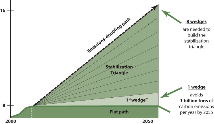
Figure 12.9b Climate Stabilization Wedges
Source: Princeton Environmental Institute, Carbon Mitigation Initiative, 2015.
Adaptation aims to reduce the public health impact of climate change. For example, if we anticipate severe weather events such as hurricanes, then preparation by emergency management authorities and medical facilities can minimize morbidity and mortality. This presupposes rigorous vulnerability assessment efforts, to identify likely events, at-risk populations, and opportunities to reduce harm (Ebi, Smith, & Burton, 2005; Kirch, Menne, & Bertollini, 2005; Menne & Ebi, 2006; Schipper & Burton, 2009).
Improving essential infrastructure could help communities adapt to climate change. For example, vegetation, building placement, white roofs, and architectural design can reduce the urban heat island effect and therefore electricity demands for air conditioning. These efforts can involve complicated trade-offs. For example, a recent study found that waste heat from air conditioning can warm outdoor air more than 1°C, so an important adaptation to urban heat islands—the use of air conditioning—can actually contribute to urban heat islands (Salamanca, Georgescu, Mahalov, Moustaoui, & Wang, 2014)! Other examples of adaptation measures include heat wave early warning systems (Lowe, Ebi, & Forsberg, 2011) and switching from surface water to groundwater sources to reduce the risk of contamination (Ebi, Lindgren, Suk, & Semenza, 2013). Optimal adaptation strategies achieve multiple objectives in tandem, taking advantage of co-benefits, as discussed on the next page.
A holistic, ecological approach to climate change adaptation, rather than engineering single solutions, may better build resiliency and secure the multiple potential benefits and cost savings associated with these improvements. As sea level rises, seawalls have frequently served to stabilize shorelines. But planting mangroves for storm surge protection incurs a fraction of the cost of building and maintaining seawalls or dikes for this purpose, while also preserving wetlands and marine food chains that support local fisheries (Arkema et al., 2013).
Public Health Action
Public health action related to climate change is based on many of the core public health functions, and utilizes many of the standard tools in the public health toolbox (Frumkin, Hess, Luber, Malilay, & McGeehin, 2008). For instance, public health surveillance is needed to detect the emergence or range expansion of infectious diseases, and public health communication helps people recognize hazards and take appropriate precautionary actions. Forecasting and modeling, which are relatively new to public health, are also central to tackling climate change. In this endeavor, public health professionals collaborate with climate scientists, demographers, and others to build scenarios predicting how climate change will affect human health. Because the effects of climate change vary from place to place, scenarios are developed for specific locations (Moss et al., 2010; Ebi et al., 2014). This in turn enables planning and implementing strategies to protect the public.
Several frameworks for public health action on climate change have been proposed. A leading example is Building Resistance Against Climate Affects, or BRACE, described in Text Box 12.2.
Co-Benefits
An important theme in both mitigation and adaptation is co-benefits. Although the steps needed to address climate change may appear formidable, some of them—reducing greenhouse gas emissions, shifting to renewable energy sources, shifting transportation patterns, shifting diets toward less meat, and others—yield many benefits (Jack & Kinney, 2010; Cheng & Berry, 2013; Thurston, 2013; West et al., 2013; Balbus, Greenblatt, Chari, Millstein, & Ebi, 2014), making them especially attractive, cost effective, and politically feasible. Examples of such co-benefits are shown in Table 12.3. Many of these co-benefits have been carefully investigated and quantified. For example, the production of meat is highly carbon intensive, accounting for as much as 18% of global greenhouse gas emissions (FAO, 2006). A British study found that lowering the consumption of red and processed meat in that country could reduce its greenhouse gas emissions by 3%, while cutting risks of coronary heart disease, diabetes, and colorectal cancer by fractions ranging up to 12% (Aston, Smith, & Powles, 2012). Similarly, a study in the Midwestern United States found that replacing short automobile trips by bicycling could reduce regional PM2.5 and ozone levels, and increase physical activity, enough to avoid 1,295 deaths per year in a region of 31.3 million people, and save approximately $3.8 billion a year from avoided mortality and reduced health care costs (Grabow et al., 2012). Such opportunities are referred to as no-regrets solutions, as suggested in Figure 12.11.
Table 12.3 Co-Benefits of Climate Mitigation and Adaptation Activities
| Climate strategies | ||||||||
| Mitigation | Adaptation | |||||||
| Shift From Single-Occupancy Vehicles Toward Cycling, Walking, Transit | Shift Diets Toward Less Meat, More Fruits and Vegetables | Shift Energy Sources From Fossil Fuels to Renewable Energy Sources | Reduced Energy Demand Through Conservation | Green Building | Urban Trees, Parks, and Green Space | Emergency Prepared-ness | ||
| Benefits | ||||||||
| Direct | Indirect | |||||||
| ↑ Physical activity | ↓ Cardiovascular disease, cancer, depression, etc. |  |
|
|||||
| ↑ Air quality | ↓ Cardiovascular & respiratory disease | |
|
|
||||
| Healthier diets | ↓ Cardiovascular disease, stroke | |
||||||
| ↑ Nature contact | ↑ Mental health, ↑ physical activity, ↑ property values |
|
|
|||||
| ↑ Social capital | ↑ Overall health and well-being | |
|
|||||
| ↓ Urban heat island | ↓ Heat-related morbidity | |
||||||
| Improved stormwater management | ↓ Flooding | |
||||||
| Economic benefits | |
|
|
|
|
|
|
|
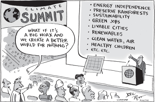
Figure 12.11 No-Regrets Solutions
Source: Pett, 2009.
Joel Pett Editorial Cartoon used with the permission of Joel Pett and the Cartoonist Group. All rights reserved.
Climate Change as a Public Issue
Public Belief in Climate Change
Perspectives on and responses to climate change vary widely. Two decades of polling suggest that about two thirds of Americans believe that climate change is occurring; of these about two thirds (or about 40% of the total) believe humans cause it, and about half (or about one in three overall) believe it will pose a serious threat in their lifetimes (Jones, 2014; Pew Research, 2014; Leiserowitz et al., 2015). Americans tend to view climate change as remote in time and space—a problem for the next generation or people in faraway countries—and rank it as a low priority, well behind concerns such as jobs, health care, or even other environmental issues (Pew Research, 2014). In other wealthy nations, climate change tends to elicit greater public concern (Pugliese & Ray, 2009; Lee, Markowitz, Howe, Ko, & Leiserowitz, 2015).
The U.S. population may be segmented along a spectrum from “alarmed” (≈16%) to “dismissive” (≈10%), according to climate change beliefs, concerns, and motivations (Roser-Renouf et al., 2014) (Figure 12.12). Many factors shape views of climate change (Brulle, Carmichael, & Jenkins, 2012): economic trends, cultural norms, the beliefs of family and friends, and values and political ideology. People often form and reinforce their beliefs using cognitive shortcuts called heuristics, which bypass evidence (Pidgeon & Fischoff, 2011). Media coverage matters (Boykoff, 2011). Deliberate, well-funded attempts to deceive the public and sow confusion have succeeded (Oreskes & Conway, 2010; Brulle, 2014); despite robust scientific consensus on climate change, there is widespread perception that scientists disagree, which in turn fuels public disbelief (Lewandowsky, Gignac, & Vaughan, 2013). Many people also are unduly influenced by personal experience, such as short-term weather perturbations. A heat wave may strengthen belief in climate change, and a snowy winter may undermine it. Interpretation of weather rests heavily on prior beliefs and social cues (T. A. Myers, Maibach, Roser-Renouf, Akerlof, & Leiserowitz, 2013; Zaval, Keenan, Johnson, & Weber, 2014).

Figure 12.12 Global Warming's Six Americas: Arraying the U.S. Population Along a Continuum of Belief, Concern, and Motivation
Source: Roser-Renouf et al., 2014.
As discussed in Chapter 28, effective communication may shift knowledge, attitudes, and behavior toward reducing risks and promoting health. This is as true for climate change as it is for other health-relevant exposures (Maibach, Roser-Renouf, & Leiserowitz, 2008), and climate communication has become a focus of research and practice in both public health and other fields (Moser & Lisa, 2007; Moser, 2010; Whitmarsh, O'Neill, & Lorenzoni, 2011; Bostrom, Böhm, & O'Connor, 2013). The salient principles are those used in environmental health communication more generally: two-way communication, gearing messages to the audience, limiting use of fear-based messages (Feinberg & Willer, 2011), frequently repeating simple, clear messages from trusted sources, and making health-promoting choices easy and appealing.
For communicating climate change, health may be a compelling frame (Maibach, Nisbet, Baldwin, Akerlof, & Diao, 2010; Myers, Nisbet, Maibach, & Leiserowitz, 2012), reflecting the fact that substantial numbers of people believe that climate change threatens health (Akerlof et al., 2010). Although further research is needed to define the role of health in climate communication, practical communication resources are becoming available (Maibach, Nisbet, & Weathers, 2011). Moreover, health care providers are a highly trusted source, ranking significantly higher than mainstream media (Leiserowitz et al., 2015), implying an important role for health professionals in climate communication.
Climate Change Policy
International efforts to address climate change are carried out under the United Nations Framework Convention on Climate Change (UNFCCC). Adopted in 1992, the UNFCCC sets out a framework that aimed to stabilize atmospheric concentrations of greenhouse gases at a level that would prevent dangerous interference with the climate system. The UNFCCC has carried out its business through regular meetings called the Conferences of Parties (COP). Perhaps the best known was the third meeting, in 1997 in Kyoto. This resulted in the Kyoto Protocol, which committed developed countries and emerging market economies to reduce their overall emissions of six greenhouse gases by at least 5% below 1990 levels over the period between 2008 and 2012, with specific targets varying from country to country. However, the United States, at the time the largest greenhouse gas emitter (China has since surpassed it), did not sign the Kyoto Protocol.
By 2007, it was clear that many signatory nations were not on track to achieve their anticipated emission reductions, even though the protocol required relatively modest emissions reductions, far below those required to stabilize greenhouse gases at any level below 700 ppm. Barriers to robust international agreements have included the unwillingness of some wealthy countries (including the United States) to accept binding limits, and tension between wealthy countries (which have caused most greenhouse gas emissions) and low- and middle-income countries (which are eager for economic development, and believe that wealthy countries should shoulder much of the responsibility).
Market mechanisms could play a powerful role in reducing carbon emissions. This involves putting a price on carbon, to correct a market failure that contributes to ongoing emissions: the fact that the costs of these emissions are not borne by the individuals and firms that benefit but instead are externalized. There are two major approaches to increasing the price of carbon, both designed to guide decision making, reduce high-carbon practices, and incentivize the development and use of low-carbon technologies. In the first, cap and trade, government sets a ceiling (or cap) on total greenhouse gas emissions and distributes emissions permits (say, through an auction) among companies that emit. Companies then buy and sell these permits at prevailing market prices, as government progressively lowers the cap to reach stated goals. The United States successfully used a cap-and-trade system to reduce sulfur dioxide and nitrous oxide emissions beginning in the 1980s, and greenhouse gas cap-and-trade systems are in place in the European Union, California, Tokyo, and other jurisdictions. The second mechanism is a carbon tax, in which government places a tax on carbon emissions. Carbon taxes are in use in Sweden and Ireland, in the Canadian provinces of British Columbia and Quebec, in Boulder, Colorado, and other jurisdictions. Economists and policy experts debate the relative merits of these two approaches (Aldy & Stavins, 2012; Goulder & Schein, 2013). While the debate may sound far removed from public health, the role of carbon pricing in preventing illness and injury makes the subject very much a matter of health policy (Howden-Chapman, Chapman, Capon, & Wilson, 2011).
However, both approaches require legislative action, and both meet stiff political opposition from such interests as fossil fuel companies (Jenkins, 2014). This political reality has prevented action at the federal level in the United States, and in Australia led to the repeal of a carbon tax in 2014, just two years after it was adopted. The alternative, then, is executive action. In the United States, this means regulation by the U.S. Environmental Protection Agency (EPA). Regulation of greenhouse gases dates to the Massachusetts v. EPA Supreme Court ruling in 2007, which found that greenhouse gases met the definition of air pollutants under the Clean Air Act. The EPA was then required to make a scientific determination—an endangerment finding—that greenhouse gas emissions were “reasonably anticipated to endanger public health or welfare.” The EPA made this determination in 2009—a striking example of climate regulation being grounded in public health. This finding, in turn, required the EPA to regulate motor vehicle greenhouse gas emissions.
Since then, the EPA has initiated a series of regulatory actions, both for mobile sources and for stationery sources, designed to reduce greenhouse gas emissions, as well as to yield other benefits. These include stricter vehicle emission standards for both light-duty vehicles (called Corporate Average Fuel Efficiency, or CAFE, standards) and trucks, and stricter emissions standards for power plants and factories.
In November, 2014, U.S. President Barack Obama and Chinese President Xi Jinping, whose nations together account for more than a third of the world's greenhouse gas emissions, announced a joint commitment on climate change. President Obama agreed to cut US CO2 emissions 28% below 2005 levels by the year 2025, and President Xi pledged that by 2030, China's CO2 emissions would peak and its share of renewable energy would rise by 20 percent. These commitments set the stage for the twenty-first COP, in Paris, in December, 2015. At that convening, nearly 200 nations agreed on the goal of limiting global warming to two degrees Centigrade, each nation agreed to set Nationally Determined Contributions toward that goal, wealthy nations agreed to help fund climate adaptation actions by poor nations, and provisions for transparency and verification were adopted. While critics noted that these steps would not suffice to avoid serious risks, most observers celebrated COP21 as a turning point and a major step forward.
Ethical Considerations
Climate change raises ethical concerns in several ways. First, on the global scale, the nations responsible for the lion's share of carbon emissions to date account for a small proportion of the world's population and are relatively resilient to the effects of climate change. In contrast, the large population of the global south—the poor countries—accounts for a relatively small share of cumulative carbon emissions, and a very low per capita emission rate (although total emissions from developing nations are growing rapidly, with China surpassing the United States in 2006). The United States, with 5% of the global population, produces 25% of total annual greenhouse gas emissions. This discrepancy exemplifies the ethical implications posed by climate change on a global scale, shown graphically in Figure 12.13. Poor populations in the developing world have little by way of industry, transportation, or intensive agriculture; they contribute only a fraction of the greenhouse gases per capita that the developed countries produce, and their capacity to protect themselves against the adverse consequences of what are mostly others' greenhouse gases is quite limited (Shue, 2014). Of course, if developing nations do not choose energy-efficient development pathways, global climate change trends will intensify even as the imbalance of equity decreases (Patz & Kovats, 2002).
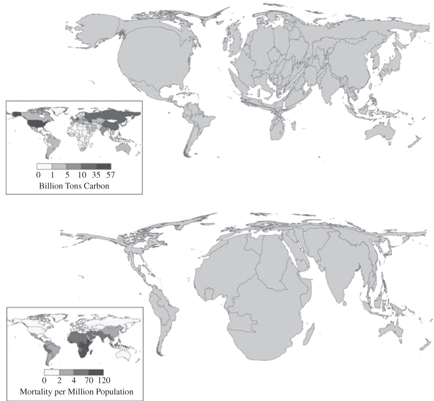
Figure 12.13 A Comparison of Cumulative CO2 Emissions (1950–2000) (upper panel) with the Burden of Four Climate-Related Health Effects (Malaria, Malnutrition, Diarrhea, and Inland Flood-Related Fatalities (lower panel)
Source: Patz, Gibbs, Foley, Rogers, & Smith, 2007.
Note the mismatch between the countries that have contributed most to climate change, and the countries that are suffering its consequences the most.
Within the United States, and within many other nations, a similar disparity exists. Poor and disadvantaged people in many cases bear the brunt of climate change impacts, including health impacts—a pattern reflecting broader inequities in environmental health, as discussed in Chapter 11. This was graphically demonstrated in the aftermath of Hurricane Katrina, a disaster typical of those expected to increase with climate change. The poor populations of New Orleans and the nearby Gulf region were disproportionately likely to fail to evacuate, to suffer catastrophic disruption following the storm, and to be unable to recover (Pastor et al., 2006; Dyson, 2007). The realization of inequities in risk and recovery resources has given rise to the concept of climate justice, a subset of environmental justice (Schlosberg & Collins, 2014).
Finally, an ethical issue arises with respect to intergenerational justice. Climate change has enormous potential impacts on the health and well-being of future generations (Page, 2007; Gardiner, 2011). As discussed in Chapter 10, ethical and religious thinkers have argued that we in the present owe a moral obligation to those who will follow to reverse climate change. For economists, the discount rate is a means of expressing value with regard to future generations. For example, the Stern report, a prominent economic analysis of climate change, used a 1.4% discount rate (Stern, 2006), whereas other economists have applied a several-fold higher discount rate (Broome, 2008). The higher discount rate implies to policymakers that the current generation should spend less on mitigating climate change, whereas the lower discount rate suggests more spending on mitigating climate change now, to avoid future harm. Policy decisions on how much the current generation should spend to mitigate climate change for the benefit of yet unborn people involve both an ethical issue and an economic issue.
Summary
Climatologists now state with high certainty that global climate change is real, occurring more rapidly than expected, and caused by human activities, especially through fossil fuel combustion and deforestation. Environmental public health researchers assessing future projections for global climate have concluded that, on balance, adverse health outcomes will dominate under these changed climatic conditions. The number of pathways through which climate change can affect the health of populations makes this environmental health threat one of the largest and most formidable of the new century. Conversely, the potential health co-benefits from moving beyond our current fossil fuel–based economy may offer some of the greatest health opportunities in recent history.
Key Terms
- adaptation
- Adjustments in ecological, social, or economic systems in response to observed or expected climate impacts. More particularly, changes in processes, practices, and structures to reduce potential harm or to exploit beneficial opportunities associated with climate change.
- adaptive management
- An iterative, learning-based approach to the design, implementation, and evaluation of interventions in complex, changing systems.
- albedo
- Reflectivity; the fraction of incident energy (such as light) reflected by a surface without being absorbed.
- cap and trade
- An environmental policy tool designed to limit emissions of a pollutant such as carbon dioxide or sulfur dioxide. The cap is a limit on emissions set by a regulatory authority; the limit is lowered over time to reduce emissions. The trade is a market for permits to emit. Using this trading, emitters able to reduce their emissions can sell their allocated permits to other emitters. This approach creates incentives to innovate to reduce emissions (cf. carbon tax).
- carbon tax
- An environmental policy tool designed to reduce carbon emissions by placing a tax on carbon emissions, generally upstream (say, at the point of fossil fuel production). By increasing the price of carbon-based fuels, a carbon tax would reduce demand (cf. cap and trade).
- climate change
- Global-scale changes resulting from higher concentrations of greenhouse gases, land-use changes such as deforestation, and other drivers. Features Earth system changes such as changes in rainfall patterns, greater ocean acidification, and more frequent heat waves. These effects vary from place to place.
- climate justice
- The concept of fairness and equity in bearing the risks of climate change and benefiting from protection against that change. A form of environmental justice.
- climate variability
- Fluctuations of climate over seasons and years relative to long-term average patterns.
- co-benefits
- Benefits that flow from an action in addition to the primary benefits that motivated the action (also called collateral benefits). For example, shifting travel from automobiles to walking, cycling, and transit is a climate mitigation strategy that also yields benefits through improved air quality, increased physical activity, and reduced road traffic fatalities.
- dangerous interference
- “Dangerous anthropogenic interference with the climate system” is the term of art used by the UNFCCC to characterize human actions that have driven earth system changes beyond a threshold of safety and stability.
- El Niño–Southern Oscillation (ENSO)
- Natural year-to-year variations in sea surface temperatures, surface air pressure, rainfall, and atmospheric circulation across the equatorial Pacific Ocean.
- endangerment finding
- The EPA's 2009 determination, under the Clean Air Act, that greenhouse gas emissions were “reasonably anticipated to endanger public health or welfare.” This finding triggered EPA regulation of greenhouse gases.
- global warming
- The increase in average surface temperature on a global scale. Climate change is a preferred term because, while warming refers only to one parameter (temperature) and one direction of change (hotter), climate change takes in the complex changes in many earth systems.
- greenhouse gases
- Atmospheric gases that increase radiative forcing: carbon dioxide, water vapor, methane, and others.
- harmful algal blooms
- Overgrowths of algae in bodies of water, usually following excess loading of nutrients into the water, and often harming aquatic ecosystems and posing health risks to people.
- heat wave
- A period of extremely hot days, defined by the World Meteorological Organization as more than five consecutive days with temperatures 5°C above the average maximum during the 1961–1990 baseline period.
- Kyoto Protocol
- A 1997 international treaty, negotiated under the UNFCCC, that committed nations to reduce greenhouse gas emissions.
- mitigation
- Actions that aim to stabilize or reduce the production of greenhouse gases (and perhaps to sequester those greenhouse gases that are produced), corresponding to the public health concept of primary prevention.
- ocean acidification
- The ongoing trend toward lower pH in the oceans, resulting from absorbing carbon dioxide.
- radiative forcing
- The difference between solar energy absorbed by the Earth and energy radiated from it.
- stabilization wedges
- Mitigation strategies that contribute to reducing greenhouse gas emissions, and that—in aggregate—achieve a designated goal.
- tail risk
- The extreme end of a distribution of probabilities for a particular outcome. In the context of climate change, tail risk corresponds to low-probability, high-consequence events such as extreme sea level rise.
- United Nations Framework Convention on Climate Change (UNFCCC)
- A framework adopted internationally in 1992 that aimed to stabilize greenhouse gases at a level that would prevent “dangerous interference” with the climate system.
- urban heat island
- An urban area that is routinely hotter than surrounding areas.
- vulnerability assessment
- Systematic, place-based evaluation of degree of exposure to hazards (susceptibility) and capacity to cope with or recover from consequences of disasters (resilience).
Discussion Questions
- Climate change has been called the major environmental health challenge of the twenty-first century. Do you agree or disagree? Explain your reasoning.
- Identify three current environmental health problems likely to be exacerbated by climate change. How might existing public health practices be altered to anticipate these effects of climate change? What other key sectors (beyond health) should be engaged?
- What are some of the major driving forces behind both the risks of climate change and our vulnerabilities to that change? Which scientific experts would be best able to assemble a comprehensive assessment of climate change risks? What types of policymakers should be involved, and at what levels (local, regional, international)?
- What are three potential co-benefits and three potential unintended consequences of mitigating greenhouse gas emissions?
- How large is your carbon footprint? Online calculators are available at these sites: www.carbonfootprint.com/calculator.aspx; www3.epa.gov/carbon-footprint-calculator; www.nature.org/greenliving/carboncalculator; and www.terrapass.com/carbon-footprint-calculator
- A substantial minority of Americans do not believe that climate change is occurring or that humans play a role. Why do you think these beliefs persist despite scientific evidence to the contrary?
- Suppose your local health department hired you to oversee climate change planning and preparedness. What steps would you take in your first sixty days on the job? In your first year?
References
- Akerlof, K., Debono, R., Berry, P., Leiserowitz, A., Roser-Renouf, C., Clarke, K. L.,…Maibach, E. W. (2010). Public perceptions of climate change as a human health risk: Surveys of the United States, Canada and Malta. International Journal of Environmental Research in Public Health, 7, 2559–2606.
- Aldy, J. E., & Stavins, R. N. (2012). Using the market to address climate change: Insights from theory & experience. Daedalus, 141(2), 45–60.
- Allergy USA. (2014). Allergy facts and figures. Retrieved from http://allergyusa.com/allergy-resources/providers/allergy-facts-figures
- Anderson, D. M., Cembella, A. D., & Hallegraeff, G. M. (2012). Progress in understanding harmful algal blooms: Paradigm shifts and new technologies for research, monitoring, and management. Annual Review of Marine Science, 4(1), 143–176.
- Arkema, K. K., Guannel, G., Verutes, G., Wood, S. A., Guerry, A., Ruckelshaus, M.,…Silver, J. M. (2013). Coastal habitats shield people and property from sea-level rise and storms. Nature Climate Change, 3(10), 913–918.
- Aston, L. M., Smith, J. N., & Powles, J. W. (2012). Impact of a reduced red and processed meat dietary pattern on disease risks and greenhouse gas emissions in the UK: A modelling study. BMJ Open, 2(5). doi:10.1136/bmjopen-2012-001072
- Bailey, R. (2011). Growing a better future: Food justice in a resource-constrained world. Oxford, U.K.: Oxfam. Retrieved from https://www.oxfam.org/en/growing-better-future
- Balbus, J. M., Greenblatt, J. B., Chari, R., Millstein, D., & Ebi, K. L. (2014). A wedge-based approach to estimating health co-benefits of climate change mitigation activities in the United States. Climatic Change, 127(2), 199–210.
- Barriopedro, D., Fischer, E. M., Luterbacher, J., Trigo, R. M., & García-Herrera, R. (2011). The hot summer of 2010: Redrawing the temperature record map of Europe. Science, 332, 220–224.
- Basu, R., & Samet, J. M. (2002). Relation between elevated ambient temperature and mortality: A review of the epidemiologic evidence. Epidemiologic Reviews, 24(2), 190–202.
- Ben-Ari, T., Neerinckx, S., Gage, K. L., Kreppel, K., Laudisoit, A., Leirs, H., & Stenseth, N. C. (2011). Plague and climate: Scales matter. PLoS Pathogens, 7(9).
- Bender, M. A., Knutson, T. R., Tuleya, R. E., Sirutis, J. J., Vecchi, G. A., Garner, S. T., & Held, I. M. (2010). Modeled impact of anthropogenic warming on the frequency of intense Atlantic hurricanes. Science, 327, 454–458.
- Bernard, S. M., Samet, J. M., Grambsch, A., Ebi, K. L., & Romieu, I. (2001). The potential impacts of climate variability and change on air pollution–related health effects in the United States. Environmental Health Perspectives, 109(Suppl. 2), 199–209.
- Berry, H. L., Bowen, K., & Kjellstrom, T. (2010). Climate change and mental health: A causal pathways framework. International Journal of Public Health, 55, 123–132.
- Berry, H. L., Hogan, A., Owen, J., Rickwood, D., & Fragar, L. (2011). Climate change and farmers' mental health: Risks and responses. Asia-Pacific Journal of Public Health, 23(2, Suppl.), 119S–132.
- Bostrom, A., Böhm, G., & O'Connor, R. E. (2013). Targeting and tailoring climate change communications. Wiley Interdisciplinary Reviews: Climate Change, 4(5), 447–455. doi:10.1002/wcc.234
- Bouchama, A., Dehbi, M., Mohamed, G., Matthies, F., Shoukri, M., & Menne, B. (2007). Prognostic factors in heat wave related deaths: A meta-analysis. Archives of Internal Medicine, 167(20), 2170–2176.
- Boykoff, M. (2011). Who speaks for the climate? Making sense of media reporting on climate change. Cambridge, U.K.: Cambridge University Press.
- Broome, J. (2008). The ethics of climate change. Scientific American, 298, 96–102.
- Brubaker, M., Berner, J., Chavan, R., & Warren, J. (2011). Climate change and health effects in northwest Alaska. Global Health Action, 4.
- Brulle, R. (2014). Institutionalizing delay: Foundation funding and the creation of U.S. climate change counter-movement organizations. Climate Change, 122, 681–694.
- Brulle, R., Carmichael, J., & Jenkins, J. C. (2012). Shifting public opinion on climate change: An empirical assessment of factors influencing concern over climate change in the U.S., 2002–2010. Climate Change, 114, 169–188.
- Bulbena, A., Sperry, L., & Cunillera, J. (2006). Psychiatric effects of heat waves. Psychiatric Services, 57(10), 1519.
- Bush, K. F., O'Neill, M. S., Li, S., Mukherjee, B., Hu, H., Ghosh, S., & Balakrishnan, K. (2014). Associations between extreme precipitation and gastrointestinal-related hospital admissions in Chennai, India. Environmental Health Perspectives, 122, 249.
- Caminade, C., Kovats, S., Rocklov, J., Tompkins, A. M., Morse, A. P., Colon-Gonzalez, F. J.,…Lloyd, S. J. (2014). Impact of climate change on global malaria distribution. Proceedings of the National Academy of Sciences of the United States of America, 111(9), 3286–3291.
- Campbell, L. P., Luther, C., Moo-Llanes, D., Ramsey, J. M., Danis-Lozano, R., & Peterson, A. T. (2015). Climate change influences on global distributions of dengue and chikungunya virus vectors. Philosophical Transactions of the Royal Society of London. Series B: Biological Sciences, 370(1665).
- Cann, K., Thomas, D. R., Salmon, R., Wyn-Jones, A., & Kay, D. (2013). Extreme water-related weather events and waterborne disease. Epidemiology and Infection, 141, 671–686.
- Carbon Dioxide Information Analysis Center. (2014). Recent greenhouse gas concentrations. doi:10.3334/CDIAC/atg.032. Retrieved from http://cdiac.ornl.gov/pns/current_ghg.html
- Centers for Disease Control and Prevention. (2013). Heat-related deaths after an extreme heat event—four states, 2012, and United States, 1999–2009. Morbidity and Mortality Weekly Report, 62(22), 433–436.
- Centers for Disease Control and Prevention. (2015). The CDC's Building Resilience Against Climate Effects (BRACE) framework. Retrieved from http://www.cdc.gov/climateandhealth/brace.htm
- Centre for Research on the Epidemiology of Disasters. (2015). The human cost of natural disasters: A global perspective. Brussels: Université Catholique de Louvain. Retrieved from http://reliefweb.int/sites/reliefweb.int/files/resources/PAND_report.pdf
- Chakraborty, S., & Newton, A. C. (2011). Climate change, plant diseases and food security: An overview. Plant Pathology, 60, 2–14.
- Checkley, W., Epstein, L. D., Gilman, R. H., Figueroa, D., Cama, R. I., Patz, J. A., & Black, R. E. (2000). Effects of El Niño and ambient temperature on hospital admissions for diarrhoeal diseases in Peruvian children. Lancet, 355, 442–450.
- Cheng, J. J., & Berry, P. (2013). Health co-benefits and risks of public health adaptation strategies to climate change: A review of current literature. International Journal of Public Health, 58(2), 305–311.
- CNA Military Advisory Board. (2014). National security and the accelerating risks of climate change. Alexandria, VA: CNA Corporation.
- Cochrane, K., De Young, C., Soto, D., & Bahri, T. (2009). Climate change implications for fisheries and aquaculture. Rome: Food and Agriculture Organization. Retrieved from http://www.fao.org/docrep/012/i0994e/0994e00.htm
- Collins, W. D., Ramaswamy, V., Schwarzkopf, M. D., Sun, Y., Portmann, R. W., Fu, Q.,…Zhong, W. Y. (2006). Radiative forcing by well-mixed greenhouse gases: Estimates from climate models in the Intergovernmental Panel on Climate Change (IPCC) Fourth Assessment Report (AR4). Journal of Geophysical Research—Atmospheres, 111, D14317. doi:10.1029/2005JD006713
- Colwell, R. R. (1996). Global climate and infectious disease: The cholera paradigm. Science, 274, 2025–2031.
- Curriero, F., Patz, J. A., Rose, J., & Lele, S. (2001). The association between extreme precipitation and waterborne disease outbreaks in the United States, 1948–1994. American Journal of Public Health, 91, 1194–1199.
- Cusack, L., de Crespigny, C., & Athanasos, P. (2011). Heatwaves and their impact on people with alcohol, drug and mental health conditions: A discussion paper on clinical practice considerations. Journal of Advanced Nursing, 67(4), 915–922.
- Davis, S. J., Cao, L., Caldeira, K., & Hoffert, M. I. (2013). Rethinking wedges. Environmental Research Letters, 8(1).
- De Man, H., van den Berg, H., Leenen, E., Schijven, J. F., Schets, F. M., van der Vliet, J. C.,…de Roda Husman, A. M. (2014). Quantitative assessment of infection risk from exposure to waterborne pathogens in urban floodwater. Water Research, 48, 90–99.
- Dhiman, R. C., Pahwa, S., Dhillon, G. P., & Dash, A. P. (2010). Climate change and threat of vector-borne diseases in India: Are we prepared? Parasitology Research, 106(4), 763–773.
- Doherty T. J., & Clayton S. (2011). The psychological impacts of global climate change. American Psychologist, 66, 265–276.
- Dunne J. P., Stouffer, R., & John, J. G. (2013). Reductions in labour capacity from heat stress under climate warming. Nature Climate Change, 3, 563–566.
- Dwight, R. H., Semenza, J. C., Baker, D. B., & Olson, B. H. (2002). Association of urban runoff with coastal water quality in Orange County, California. Water Environment Research, 74(1), 82–90.
- Dyson, M. E. (2007). Come hell or high water: Hurricane Katrina and the color of disaster. New York: Basic Books.
- Ebi, K. L., Hallegatte, S., Kram, T., Arnell, N., Carter, T., Edmonds, J.,…Zwickel, T. (2014). A new scenario framework for climate change research: Background, process, and future directions. Climatic Change, 122(3), 363–372.
- Ebi, K. L., Lindgren, E., Suk, J. E., & Semenza, J. C. (2013). Adaptation to the infectious disease impacts of climate change. Climatic Change, 118(2), 355–365.
- Ebi, K. L., Smith, J., & Burton, I. (Eds.). (2005). Integration of public health with adaptation to climate change: Lessons learned and new directions. London: Taylor & Francis.
- El-Fadel, M., Ghanimeh, S., Maroun, R., & Alameddine, I. (2012). Climate change and temperature rise: Implications on food- and water-borne diseases. Science of the Total Environment, 437, 15–21.
- Feinberg, M., & Willer, R. (2011). Apocalypse soon? Dire messages reduce belief in global warming by contradicting just-world beliefs. Psychological Science, 22(1), 34–38.
- Fiore, A. M., Naik, V., & Leibensperger, E. M. (2015). Air quality and climate connections. Journal of the Air & Waste Management Association, 65(6).
- Fisher, G. T., & Katz, B. G. (1988). Urban stormwater runoff: Selected background information and techniques for problem assessment with a Baltimore, Maryland, case study (U.S. Geological Survey Water-Supply Paper 2347). Reston, VA: U.S. Geological Survey.
- Food and Agriculture Organization of the United Nations. (2006). Livestock's long shadow: Environmental issues and options. Rome: Author. Retrieved from http://www.fao.org/docrep/010/a0701e/a0701e00.HTM
- Food and Agriculture Organization of the United Nations. (2013). The state of food insecurity in the world 2013: The multiple dimensions of food security. Rome: Author.
- Fritze, J. G., Blashki, G. A., Burke, S., & Wiseman, J. (2008). Hope, despair and transformation: Climate change and the promotion of mental health and wellbeing. International Journal of Mental Health Systems, 2(1), 13.
- Frumkin, H., Hess, J., Luber, G., Malilay, J., & McGeehin, M. (2008). Climate change: The public health response. American Journal of Public Health, 98, 435–445.
- Frumkin, H., & McMichael, A. J. (2008). Climate change and public health: Thinking, communicating, acting. American Journal of Preventive Medicine, 35, 403–410.
- Fu, F. X., Tatters, A. O., & Hutchins, D. A. (2012). Global change and the future of harmful algal blooms in the ocean. Marine Ecology Progress Series, 470, 207–233.
- Galea, S., Brewin, C. R., Gruber, M., Jones, R. T., King, D. W., King, L. A.,…Kessler, R. C. (2007). Exposure to hurricane-related stressors and mental illness after Hurricane Katrina. Archives of General Psychiatry, 64, 1427–1434.
- Gardiner, S. M. (2011). A perfect moral storm: The ethical tragedy of climate change. New York: Oxford University Press.
- Gingold, D. B., Strickland, M. J., & Hess, J. J. (2014). Ciguatera fish poisoning and climate change: Analysis of National Poison Center data in the United States, 2001–2011. Environmental Health Perspectives, 122(6), 580–586.
- Glass, G. E., Cheek, J. E., Patz, J. A., Shields, T. M., Doyle, T. J., Thoroughman, D. A.,…Bryan, R. (2000). Using remotely sensed data to identify areas of risk for hantavirus pulmonary syndrome. Emerging Infectious Diseases, 63(3), 238–247.
- Glibert, P. M., Icarus Allen, J., Artioli, Y., Beusen, A., Bouwman, L., Harle, J.,…Holt, J. (2014). Vulnerability of coastal ecosystems to changes in harmful algal bloom distribution in response to climate change: Projections based on model analysis. Global Change Biology, 20(12), 3845–3858.
- Goldmann, E., & Galea, S. (2014). Mental health consequences of disasters. Annual Review of Public Health, 35, 169–183.
- Goodess, C. M. (2013). How is the frequency, location and severity of extreme events likely to change up to 2060? Environmental Science & Policy, 27, S4–14.
- Goulder, L. H., & Schein, A. (2013). Carbon taxes vs. cap and trade: A critical review. Cambridge, MA: National Bureau of Economic Research.
- Grabow M. L., Spak, S. N., Holloway, T., Stone, B., Mednick, A. C., & Patz, J. A. (2012). Air quality and exercise-related health benefits from reduced car travel in the midwestern United States. Environmental Health Perspectives, 120, 68–76.
- Gubler, D. J., Reiter, P., Ebi, K. L., Yap, W., Nasci, R., & Patz, J. A. (2001). Climate variability and change in the United States: Potential impacts on vector- and rodent-borne diseases. Environmental Health Perspectives, 109(Suppl. 2), 223–233.
- Habeeb, D., Vargo, J., & Stone, B. (2015). Rising heat wave trends in large US cities. Natural Hazards, 76(3), 1651–1665.
- Harvey, M., & Pilgrim, S. (2011). The new competition for land: Food, energy, and climate change. Food Policy, 36(Suppl. 1), S40–51.
- Hellberg, R. S., & Chu, E. (2015). Effects of climate change on the persistence and dispersal of foodborne bacterial pathogens in the outdoor environment: A review. Critical Reviews in Microbiology, 1–25. Advance online publication.
- Hess, J. J., Malilay, J. N., & Parkinson, A. J. (2008). Climate change: The importance of place. American Journal of Preventive Medicine, 35, 468–478.
- HLPE. (2013). Biofuels and food security. A Report by the High Level Panel of Experts on Food Security and Nutrition of the Committee on World Food Security. Rome: Committee on World Food Security.
- Howden-Chapman, P. L., Chapman, R. B., Capon, A. G., & Wilson, N. (2011). Carbon pricing is a health protection policy. Medical Journal of Australia, 195(6), 311–312.
- Hsiang, S. M., Burke, M., & Miguel, E. (2013). Quantifying the influence of climate on human conflict. Science, 341.
- Hurley, W., Wolterstorff, C., MacDonald, R., & Schultz, D. (2014). Paralytic shellfish poisoning: A case series. Western Journal of Emergency Medicine, 15(4), 378–381.
- Intergovernmental Panel on Climate Change. (2013). Climate change 2013: The physical science basis. Contribution of Working Group I to the Fifth Assessment Report of the Intergovernmental Panel on Climate Change. New York: Cambridge University Press.
- Jack, D. W., & Kinney, P. L. (2010). Health co-benefits of climate mitigation in urban areas. Current Opinion in Environmental Sustainability, 2, 172–177.
- Jacob, B., Mawson, A. R., Payton, M., & Guignard, J. C. (2008). Disaster mythology and fact: Hurricane Katrina and social attachment. Public Health Reports, 123, 555–566.
- Jenkins, J. D. (2014). Political economy constraints on carbon pricing policies: What are the implications for economic efficiency, environmental efficacy, and climate policy design? Energy Policy, 69, 467–477.
- Johnston F. H., Henderson, S. B., Chen, Y., Randerson, J. T., Marlier, M., Defries, R. S.,…Brauer, M. (2012). Estimated global mortality attributable to smoke from landscape fires. Environmental Health Perspectives, 120, 695–701.
- Jones, J. (2014). In U.S., most do not see global warming as serious threat: Nearly two in three believe global warming will happen during their lifetimes. Retrieved from http://www.gallup.com/poll/167879/not-global-warming-serious-threat.aspx
- Kalkstein, L. S., Greene, S., Mills, D. M., & Samenow, J. (2011). An evaluation of the progress in reducing heat-related human mortality in major U.S. cities. Natural Hazards, 56(1), 113–129.
- Kilbourne, E. M. (2008). Temperature and health. In R. B. Wallace (Ed.), Maxcy-Rosenau-Last public health and preventive medicine (15th ed., pp. 725–734). New York: McGraw-Hill Medical.
- Kirch, W., Menne, B., & Bertollini, R. (Eds.). (2005). Extreme weather events and public health responses. New York: Springer.
- Kjellstrom, T., Holmer, I., & Lemke, B. (2009). Workplace heat stress, health and productivity—an increasing challenge for low and middle-income countries during climate change. Global Health Action, 2. doi:10.3402/gha.v2i0.2047
- Kovats, R. S., Edwards, S. J., Hajat, S., Armstrong, B. G., Ebi, K. L., & Menne, B. (2004). The effect of temperature on food poisoning: A time-series analysis of salmonellosis in ten European countries. Epidemiology and Infection, 132(3), 443–453.
- Kunkel, K. E., Easterling, D. R., Redmond, K., & Hubbard, K. (2003). Temporal variations of extreme precipitation events in the United States: 1895–2000. Geophysical Research Letters, 30, 1900.
- Lake, I. R., Gillespie, I. A., Bentham, G., Nichols, G. L., Lane, C., Adak, G. K., & Threlfall, E. J. (2009). A re-evaluation of the impact of temperature and climate change on foodborne illness. Epidemiology and Infection, 137(11), 1538–1547.
- Lang-Yona, N., Levin, Y., Dannemiller, K. C., Yarden, O., Peccia, J., & Rudich, Y. (2013). Changes in atmospheric CO2 influence the allergenicity of Aspergillus fumigatus. Global Change Biology, 19(8), 2381–2388.
- Lau, C. L., Smythe, L. D., Craig, S. B., & Weinstein, P. (2010). Climate change, flooding, urbanisation and leptospirosis: Fuelling the fire? Transactions of the Royal Society of Tropical Medicine and Hygiene, 104(10), 631–638.
- Lee, T. M., Markowitz, E. M., Howe, P. D., Ko, C.-Y., & Leiserowitz, A. A. (2015). Predictors of public climate change awareness and risk perception around the world. Nature Climate Change, 5. Advance online publication. doi:10.1038/nclimate2728
- Leiserowitz, A., Maibach, E., Roser-Renouf, C., Feinberg, G., & Rosenthal, S. (2015). Climate change in the American mind: March 2015. Yale University and George Mason University. New Haven, CT: Yale Project on Climate Change Communication. Retrieved from http://environment.yale.edu/climate-communication/files/Global-Warming-CCAM-March-2015.pdf
- Levy, B. S., & Sidel, V. W. (2014). Collective violence caused by climate change and how it threatens health and human rights. Health and Human Rights International Journal, 16, 32–40.
- Lewandowsky, S., Gignac, G. E., & Vaughan, S. (2013). The pivotal role of perceived scientific consensus in acceptance of science. Nature Climate Change, 3(4), 399–404.
- Lloyd, S. J., Sari Kovats, R., & Chalabi, Z. (2011). Climate change, crop yields, and undernutrition: Development of a model to quantify the impact of climate scenarios on child undernutrition. Environmental Health Perspectives, 119, 1817–1823.
- Loughry, M. (2010). Climate change, human movement and the promotion of mental health: What have we learnt from earlier global stressors? In J. McAdam (Ed.), Climate change and displacement: Multidisciplinary perspectives (pp. 221–238). Oxford, U.K.: Hart.
- Lowe, D., Ebi, K. L., & Forsberg, B. (2011). Heatwave early warning systems and adaptation advice to reduce human health consequences of heatwaves. International Journal of Environmental Research and Public Health, 8(12), 4623–4648.
- Luber, G., Knowlton, K., Balbus, J., Frumkin, H., Hayden, M., Hess, J.,…Ziska, L. (2014). Human health. In J. M. Melillo, T. C. Richmond, & G. W. Yohe (Eds.), Climate change impacts in the United States: The third national climate assessment (pp. 220–256). U.S. Global Change Research Program. Washington, DC: U.S. Government Printing Office.
- Luber G., & McGeehin M. (2008). Climate change and extreme heat events. American Journal of Preventive Medicine, 35, 429–435.
- Maibach, E. W., Nisbet, M., Baldwin, P., Akerlof, K., & Diao, G. (2010). Reframing climate change as a public health issue: An exploratory study of public reactions. BMC Public Health, 10, 299.
- Maibach, E., Nisbet, M., & Weathers, M. (2011). Conveying the human implication of climate change: A climate change communication primer for public health professionals. Fairfax, VA: George Mason University Center for Climate Change Communication. Retrieved from http://www.climatechangecommunication.org/report/new-climate-change-communication-primer-public-health-professionals
- Maibach, E. W., Roser-Renouf, C., & Leiserowitz, A. (2008). Communication and marketing as climate change–intervention assets: A public health perspective. American Journal of Preventive Medicine, 35(5), 488–500.
- Marinucci, G. D., Luber, G., Uejio, C. K., Saha, S., & Hess, J. J. (2014). Building resilience against climate effects—a novel framework to facilitate climate readiness in public health agencies. International Journal of Environmental Research and Public Health, 11(6), 6433–6458.
- Martin, V., Chevalier, V., Ceccato, P., Anyamba, A., De Simone, L., Lubroth, J.,…Domenech, J. (2008). The impact of climate change on the epidemiology and control of Rift Valley fever. Revue Scientifique et Technique, 27(2), 413–426.
- Martinez, M., Devenport, L., Saussy, J., & Martinez, J. (2002). Drug-associated heat stroke. Southern Medical Journal, 95(8), 799–802.
- Matsueda, M. (2011). Predictability of Euro-Russian blocking in summer of 2010. Geophysical Research Letters, 38(6). doi:10.1029/2010GL046557
- McCarthy, J., Canziani, O. F., Leary, N. A., Dokken, D. J., & White, K. S. (Eds.). (2001). Climate change 2001: Impacts, adaptation, and vulnerability. Contribution of Working Group II to the Third Assessment Report of the Intergovernmental Panel on Climate Change. New York: Cambridge University Press.
- McLaughlin, J. B., DePaola, A., Bopp, C. A., Martinek, K. A., Napolilli, N. P., Allison, C. G.,…Middaugh, J. P. (2005). Outbreaks of Vibrio parahaemolyticus gastroenteritis associated with Alaskan oysters. New England Journal of Medicine, 353(14), 1463–1470.
- McMichael, A. J. (2013). Globalization, climate change, and human health. New England Journal of Medicine, 369(1), 96.
- McMichael, A. J., McMichael, C., Berry, H., & Bowen, K. (2010). Climate-related displacement: Health risks and responses. In J. McAdam (Ed.), Climate change and population displacement: Multidisciplinary perspectives (pp. 191–220). Oxford, U.K.: Hart.
- Medlock, J. M., & Leach, S. A. (2015). Effect of climate change on vector-borne disease risk in the UK. Lancet: Infectious Diseases, 15(6), 721–730.
- Menne, B., & Ebi, K. L. (Eds.). (2006). Climate change and adaptation strategies for human health. Darmstadt, Germany: Steinkopff-Verlag.
- Mills, J. N., Gage, K. L., & Khan, A. S. (2010). Potential influence of climate change on vector-borne and zoonotic diseases: A review and proposed research plan. Environmental Health Perspectives, 118, 1507–1514.
- Mohan, J.,E., Ziska, L. H., Schlesinger, W. H., Thomas, R. B., Sicher, R. C., George, K., & Clark, J. S. (2006). Biomass and toxicity responses of poison ivy (Toxicodendron radicans) to elevated atmospheric CO2. Proceedings of the National Academy of Sciences of the United States of America, 103(24), 9086–9089.
- Morin, C. W., Comrie, A. C., & Ernst, K. (2013). Climate and dengue transmission: Evidence and implications. Environmental Health Perspectives, 121(11–12), 1264–1272.
- Moritz, M. A., Parisien, M.-A., Batllori, E., Krawchuk, M. A., Van Dorn, J., Ganz, D. J., & Hayhoe, K. (2012). Climate change and disruptions to global fire activity. Ecosphere, 3(6), art49.
- Moser, S. C. (2010). Communicating climate change: History, challenges, process and future directions. Wiley Interdisciplinary Reviews: Climate Change, 1(1), 31–53.
- Moser, S. C., & Lisa, D. (2007). Creating a climate for change: Communicating climate change and facilitating social change. Cambridge, U.K.: Cambridge University Press.
- Moss, R. H., Edmonds, J. A., Hibbard, K. A., Manning, M. R., Rose, S. K., van Vuuren, D. P.,…Wilbanks, T. J. (2010). The next generation of scenarios for climate change research and assessment. Nature, 463(7282), 747–756.
- Murray, C.J.L., Rosenfeld, L. C., Lim, S. S., Andrews, K. G., Foreman, K. J., Haring, D.,…Lopez, A. D. (2012). Global malaria mortality between 1980 and 2010: A systematic analysis. Lancet, 379(9814), 413–431.
- Myers, S. S., Zanobetti, A., Kloog, I., Huybers, P., Leakey, A. D., Bloom, A. J.,…Usui, Y. (2014). Increasing CO2 threatens human nutrition. Nature, 510, 139–142.
- Myers, T. A., Maibach, E. W., Roser-Renouf, C., Akerlof, K., & Leiserowitz, A. A. (2013). The relationship between personal experience and belief in the reality of global warming. Nature Climate Change, 3(4), 343–347.
- Myers, T. A., Nisbet, M., Maibach, E., & Leiserowitz, A. (2012). A public health frame arouses hopeful emotions about climate change. Climate Change, 113(3–4), 1105–1112.
- National Climatic Data Center. (1999). Mitch: The deadliest Atlantic hurricane since 1780. Retrieved from http://www.ncdc.noaa.gov/ol/reports/mitch/mitch.html
- National Oceanic and Atmospheric Administration. (2014). NOAA, partners predict significant harmful algal bloom in western Lake Erie this summer. Retrieved from http://www.noaanews.noaa.gov/stories2014/20140710_erie_hab.html
- National Snow & Ice Data Center. (2015). Sea ice: More information. Retrieved from http://nsidc.org/soac/sea-ice-more-information
- Naumova, E. N., Jagai, J. S., Matyas, B., DeMaria, A., Jr., MacNeill, I. B., & Griffiths, J. K. (2007). Seasonality in six enterically transmitted diseases and ambient temperature. Epidemiology and Infection, 135(2), 281–292.
- Nelson, G. C., Rosegrant, M. W., Koo, J., Robertson, R. D., Sulser, T., Zhu, T.,…Lee, D. R. (2009). Climate change: Impact on agriculture and costs of adaptation. Washington, DC: International Food Policy Research Institute. Retrieved from http://www.ifpri.org/publication/climate-change-impact-agriculture-and-costs-adaptation
- Norris, F. H., Tracy, M., & Galea, S. (2009). Looking for resilience: Understanding the longitudinal trajectories of responses to stress. Social Science & Medicine, 68, 2190–2198.
- North, C. S., & Pfefferbaum, B. (2013). Mental health response to community disasters: A systematic review. JAMA, 310, 507–518.
- Ogden, N. H., Maarouf, A, Barker, I. K., Bigras-Poulin, M., Lindsay, L. R., Morshed, M. G.,…Charron, D. F. (2006). Climate change and the potential for range expansion of the Lyme disease vector Ixodes scapularis in Canada. International Journal for Parasitology, 36(1), 63–70.
- Oldham R. L. (2013). Mental health aspects of disasters. Southern Medical Journal, 106, 115–119.
- Oreskes, N., & Conway, E. M. (2010). Merchants of doubt. New York: Bloomsbury.
- Ostfeld, R. S., & Brunner, J. L. (2015). Climate change and Ixodes tick-borne diseases of humans. Philosophical Transactions of the Royal Society of London. Series B: Biological Sciences, 370(1665).
- Pacala, S., & Socolow, R. (2004). Stabilization wedges: Solving the climate problem for the next 50 years with current technologies. Science, 305(5686), 968–972.
- Page, E. A. (2007). Climate change, justice and future generations. Northampton, MA: Elgar.
- Page, L. A., Hajat, S., & Kovats, R. S. (2007). Relationship between daily suicide counts and temperature in England and Wales. British Journal of Psychiatry, 191, 106–112.
- Parham, P. E., Waldock, J., Christophides, G. K., Hemming, D., Agusto, F., Evans, K. J.,…Michael, E. (2015). Climate, environmental and socio-economic change: Weighing up the balance in vector-borne disease transmission. Philosophical Transactions of the Royal Society of London. Series B: Biological Sciences, 370(1665).
- Pascual, M., Ahumada, J. A., Chaves, L. F., Rodó, X., & Bouma, M. (2006). Malaria resurgence in the east African highlands: Temperature trends revisited. Proceedings of the National Academy of Sciences of the United States of America, 103(15), 5829–5834.
- Pascual, M., Rodó, X., Ellner, S. P., Colwell, R., Bouma, M. J. (2000). Cholera dynamics and El Niño–Southern Oscillation. Science, 289, 1766–1769.
- Pastor, M., Bullard, R., Boyce, J., Fothergill, A., Morello-Frosch, R., & Wright, B. (2006). In the wake of the storm: Environment, disaster, and race after Katrina. New York: Russell Sage Foundation.
- Patz, J. A., Frumkin, H., Holloway, T., Vimont, D. J., & Haines, A. (2014). Climate change: Challenges and opportunities for global health. JAMA, 312(15), 1565–1580.
- Patz, J. A., Gibbs, H. K., Foley, J. A., Rogers, J. V., & Smith, K. R. (2007). Climate change and global health: Quantifying a growing ethical crisis. EcoHealth, 4, 397–405.
- Patz, J. A., Githeko, A. K., McCarty, J. P., Hussein, S., Confalonieri, U., & de Wet, N. (2003). Climate change and infectious diseases. In A. J. McMichael, D. H. Campbell-Lendrum, C. F. Corvalán, K. L. Ebi, A. Githeko, J. D. Scheraga, & A. Woodward (Eds.), Climate change and human health: Risks and responses (pp. 103–132) Geneva: World Health Organization.
- Patz, J. A., & Hahn M. B. (2013). Climate change and human health: A One Health approach. In J. S. Mackenzie, M. Jeggo, P. Daszak, & J. A. Richt (Eds.), One Health: The human-animal-environment interfaces in emerging infectious diseases (pp. 141–171). New York: Springer.
- Patz, J. A., & Kovats, R. S. (2002). Hotspots in climate change and human health. BMJ, 325, 1094–1098.
- Patz, J. A., Vavrus, S. J., Uejio, C. K., & McLellan, S. L. (2008). Climate change and waterborne disease risk in the Great Lakes region of the U.S. American Journal of Preventive Medicine, 35, 451–458.
- Paz, S. (2015). Climate change impacts on West Nile virus transmission in a global context. Philosophical Transactions of the Royal Society of London. Series B: Biological Sciences, 370(1665).
- Petkova, E. P., Bader, D. A., Anderson, G. B., Horton, R. M., Knowlton, K., & Kinney, P. L. (2014). Heat-related mortality in a warming climate: Projections for 12 U.S. cities. International Journal of Environmental Research and Public Health, 11(11), 11371–11383.
- Pett, J. (2009). [Editorial cartoon by Joel Pett]. USA Today, December 13.
- Pew Research. (2014). Climate change: Key data points from Pew Research. Retrieved from http://www.pewresearch.org/key-data-points/climate-change-key-data-points-from-pew-research
- Pidgeon N., & Fischhoff, B. (2011). The role of social and decision sciences in communicating uncertain climate risks. Nature Climate Change, 1, 35–41.
- Porter, J. R., Xie, L., Challinor, A. J., Cochrane, K., Howden, M., Iqbal, M. M.,…Travasso, M. I. (2014). Food security and food production systems. In C. B. Field, V. R. Barros, D. J. Dokken, K. J. Mach, M. D. Mastrandrea, T. E. Bilir,…L. L. White (Eds.), Climate change 2014: Impacts, adaptation and vulnerability. Part A: Global and sectoral aspects. Contribution of Working Group II to the Fifth Assessment Report of the Intergovernmental Panel on Climate Change (pp. 485–533). New York: Cambridge University Press.
- Princeton Environmental Institute, Carbon Mitigation Initiative. (2015). Princeton, NJ: Princeton University. Retrieved from http://cmi.princeton.edu/wedges/slides.php
- Pugliese, A., & Ray, J. (2009). A heated debate: Global attitudes toward climate change. Harvard International Review, 31, 64–68.
- Robine, J.-M., Cheung, S. L., Le Roy, S., Van Oyen, H., Griffiths, C., Michel, J. P., & Herrmann, F. R. (2008). Death toll exceeded 70,000 in Europe during the summer of 2003. Comptes Rendus Biologies, 331, 171–178.
- Rodó, X., Pascual, M., Fuchs, G., & Faruque, A. S. (2002). ENSO and cholera: A nonstationary link related to climate change? Proceedings of the National Academy of Sciences of the United States of America, 99(20), 12901–12906.
- Rose, J. B. (1997). Environmental ecology of cryptosporidium and public health implications. Annual Review of Public Health, 18(1), 135–161.
- Roser-Renouf, C., Maibach, E., Leiserowitz, A., Feinberg, G., Rosenthal, S., & Kreslake, J. (2014). Global warming's six Americas, October 2014: Perception of the health consequences of global warming and update on key beliefs. Yale University and George Mason University. New Haven, CT: Yale Project on Climate Change Communication.
- Rubio, M. A., & Lissi, E. A. (2014). Temperature as thumb rule predictor of ozone levels in Santiago de Chile ground air. Journal of the Chilean Chemical Society, 59, 2427–2431.
- Running, S. W. (2006). Is global warming causing more, larger wildfires? Science, 313, 927–928.
- Salamanca, F., Georgescu, M., Mahalov, A., Moustaoui, M., & Wang, M. (2014), Anthropogenic heating of the urban environment due to air conditioning. Journal of Geophysical Research: Atmospheres, 119, 5949–5965.
- Schipper, E. L., & Burton, I. (Eds.). (2009). The Earthscan reader on adaptation to climate change. London: Earthscan.
- Schlosberg, D., & Collins, L. B. (2014). From environmental to climate justice: Climate change and the discourse of environmental justice. Wiley Interdisciplinary Reviews: Climate Change, 5(3), 359–374.
- Schuster, C. J., Ellis, A. G., Robertson, W. J., Charron, D. F., Aramini, J. J., Marshall, B. J., & Medeiros, D. T. (2005). Infectious disease outbreaks related to drinking water in Canada, 1974–2001. Canadian Journal of Public Health, 96(4), 254–258.
- Shue, H. (2014). Climate justice: Vulnerability and protection. New York: Oxford University Press.
- Socolow, R. (2011, September 27). Wedges reaffirmed [Web log post]. Retrieved from http://www.climatecentral.org/blogs/wedges-reaffirmed
- Squire, O. J., Archibald, A. T., Griffiths, P. T., Jenkin, M. E., Smith, D., & Pyle, J. A. (2015). Influence of isoprene chemical mechanism on modelled changes in tropospheric ozone due to climate and land use over the 21st century. Atmospheric Chemistry and Physics, 15(9), 5123–5143.
- Stenseth, N. C., Samia, N. I., Viljugrein, H., Kausrud, K. L., Begon, M., Davis, S.,…Chan, K. S. (2006). Plague dynamics are driven by climate variation. Proceedings of the National Academy of Sciences of the United States of America, 103(35), 13110–13115.
- Stern, N. H. (2007). The economics of climate change: The Stern review. New York: Cambridge University Press.
- Sung, T.-I., Chen, M.-J., Lin, C.-Y., Lung, S.-C., & Su, H.-J. (2011). Relationship between mean daily ambient temperature range and hospital admissions for schizophrenia: Results from a national cohort of psychiatric inpatients. Science of the Total Environment, 410–411, 41–46.
- Thompson, J. R., Randa, M. A., Marcelino, L. A., Tomita-Mitchell, A., Lim, E., & Polz, M. F. (2004). Diversity and dynamics of a North Atlantic coastal Vibrio community. Applied and Environmental Microbiology, 70(7), 4103–4110.
- Thurston, G. D. (2013). Mitigation policy: Health co-benefits. Nature Climate Change, 3(10), 863–864.
- Tirado, M. C., Cohen, M. J., Aberman, N., Meerman, J., & Thompson, B. (2010). Addressing the challenges of climate change and biofuel production for food and nutrition security. Food Research International, 43(7), 1729–1744.
- Uejio, C. K., Yale, S. H., Malecki, K., Borchardt, M. A., Anderson, H. A., & Patz, J. A. (2014). Drinking water systems, hydrology, and childhood gastrointestinal illness in central and northern Wisconsin. American Journal of Public Health, 104, 639–646.
- United Nations High Commissioner for Refugees. (2009). Climate change, natural disasters and human displacement: A UNHCR perspective. Retrieved from http://www.unhcr.org/refworld/docid/4a8e4f8b2.html
- U.S. Department of Defense. (2014). 2014 Climate change adaptation roadmap. Retrieved from http://www.acq.osd.mil/ie/download/CCARprint_wForeword_c.pdf
- Vezzulli, L., Colwell, R. R., & Pruzzo, C. (2013). Ocean warming and spread of pathogenic vibrios in the aquatic environment. Microbial Ecology, 65(4), 817–825.
- Vinck, P. (2013). World disasters report: Focus on technology and the future of humanitarian action. Geneva: International Federation of Red Cross and Red Crescent Societies. Retrieved from http://worlddisastersreport.org/en
- Weaver, S. C., & Reisen, W. K. (2010). Present and future arboviral threats. Antiviral Research, 85(2), 328–345.
- West, J. J., Smith, S. J., Silva, R. A., Naik, V., Zhang, Y., Adelman, Z.,…Lamarque, J.-F. (2013). Co-benefits of mitigating global greenhouse gas emissions for future air quality and human health. Nature Climate Change, 3, 885–889.
- Westerling, A. L., Hidalgo, H. G., Cayan, D. R., & Swetnam, T. W. (2006). Warming and earlier spring increase western U.S. forest wildfire activity. Science, 313, 940–943.
- Wheeler, T., & von Braun, J. (2013). Climate change impacts on global food security. Science, 341, 508–513.
- Whiteford, H. A., Degenhardt, L., Rehm, J., Baxter, A. J., Ferrari, A. J., Erskine, H. E.,…Vos, T. (2013). Global burden of disease attributable to mental and substance use disorders: Findings from the Global Burden of Disease Study 2010. Lancet, 382, 1575–1586.
- Whitmarsh, L., O'Neill, S., & Lorenzoni, L. (Eds.). (2011). Engaging the public with climate change: Behavior change and communication. London: Earthscan.
- WikiMedia Commons. (2011). Urban heat island profile. Retrieved from http://commons.wikimedia.org/wiki/File:Urban_heat_island_profile.gif
- Zaval, L., Keenan, E. A., Johnson, E. J., & Weber, E. U. (2014). How warm days increase belief in global warming. Nature Climate Change, 4(2), 143–147.
- Zhang, Y., Bielory, L., Mi, Z., Cai, T., Robock, A., & Georgopoulos, P. (2015). Allergenic pollen season variations in the past two decades under changing climate in the United States. Global Change Biology, 21(4), 1581–1589.
- Ziska, L. H. (2003). Evaluation of the growth response of six invasive species to past, present and future atmospheric carbon dioxide. Journal of Experimental Botany, 54(381), 395–404.
- Ziska L., Knowlton K., Rogers C., Dalan, D., Tierney, N., Elder, M. A.,…Frenz, D. (2011). Recent warming by latitude associated with increased length of ragweed pollen season in central North America. Proceedings of the National Academy of Sciences of the United States of America, 108, 4248–4251.
- Ziska, L. H., & McConnell, L. L. (2015). Climate change, carbon dioxide, and pest biology: Monitor, mitigate, manage. Journal of Agricultural and Food Chemistry. doi:10.1021/jf506101h
For Further Information
Review Articles
- McMichael, A. J. (2013). Globalization, climate change, and human health. New England Journal of Medicine, 368(14), 1335–1343.
- Patz, J. A., Frumkin, H., Holloway, T., Vimont, D. J., & Haines, A. (2014). Climate change: Challenges and opportunities for global health. JAMA, 312(15), 1565–1580.
Reports
- Intergovernmental Panel on Climate Change (IPCC): http://www.ipcc.ch. IPCC reports represent some of the most authoritative and exhaustive synthesis assessments. Its fifth assessment report was published in 2014. Full and summary reports and downloadable graphs and figures are available from the IPCC Web site.
- U.S. Centers for Disease Control and Prevention: http://www.cdc.gov/climateandhealth. This site focuses specifically on health aspects of climate change, including public health actions in response.
- U.S. Environmental Protection Agency (EPA): http://www.epa.gov/climatechange/effects/health.html. This informative EPA site covers the many sectors affected by climate change.
- U.S. Global Change Research Program: This initiative publishes periodic National Climate Assessments under the title Climate Change Impacts in the United States. The most recent assessment was published in 2014. It is available at http://nca2014.globalchange.gov
- World Health Organization (WHO): http://www.who.int/globalchange/climate/en. The WHO has been assessing the health risks of climate change for nearly two decades, and this Web site contains links to WHO reports and ongoing projects.
Books
- Butler, C. D. (Ed.). (2014). Climate change and global health. Boston: CABI.
- Epstein, P., & Ferber, D. (2011). Changing planet, changing health: How the climate crisis threatens our health and what we can do about it. Berkeley: University of California Press.
- Griffiths, J., Rao, M., Adshead, F., & Thorpe, A. (Eds.). (2009). The health practitioner's guide to climate change: Diagnosis and cure. London: Earthscan.
- Levy, B. S., & Patz, J. A. (Eds.). (2015). Climate change and public health. New York: Oxford University Press.
- Luber, G., & Lemery, J. (Eds.). (2015). Global Climate change and human health: From Science to Practice. San Francisco: Jossey-Bass.
Blogs
- Dot Earth: http://dotearth.blogs.nytimes.com. An interactive blog that explores trends and ideas with readers and experts. World-renowned reporter Andrew C. Revkin carefully follows and reports on climate change science and policy.
- RealClimate: http://www.realclimate.org. A blog containing commentaries by climate scientists that sort out the often polarizing or conflicting stories in the mainstream press. Discussions are restricted to climate science topics (and not political or economic implications). Postings are signed by the author(s) so you know exactly from where the information comes.
Materials for Teachers
- EcoHealth: http://ecohealth101.org. A source of useful information and student exercises for middle and high school teachers and students. Topics (and lesson plans) include human health effects of climate change, ozone depletion, biodiversity and land-use change, mechanized intensive agriculture, and globalization.
- GRID-Arendal: http://www.grida.no. A collaborating center of UNEP. The mission of this site (established in 1989 by the government of Norway) is to communicate environmental information to policymakers and facilitate environmental decision making for change.