
1. Age-structured models: Life tables and the Leslie matrix
2. Stage-structured matrix models
4. Continuous-time models with age structure
5. Applications and extensions
When all individuals in a population are identical, we can characterize the population just by counting the number of individuals. However, the individuals within many animal and plant populations differ in important ways that influence their current and future prospects of survival and reproduction. For example, larger individuals typically have greater chances of survival, produce more and sometimes larger offspring, and often have slower growth rates. In such cases, characterizing the population structure—the numbers of individuals of each different type—is critical for understanding how the population will change through time. In this chapter, we examine some of the main types of models used for describing and forecasting the dynamics of structured populations. Age-structured models in discrete time, appropriate for populations in seasonal environments, were developed centuries ago by the great mathematician Leonhard Euler [1707–1783]. These are considered first, before moving to models where individuals are characterized by their stage in the life cycle [e.g., seed versus flowering plant, larva versus adult). Next we look at how to incorporate differences among individuals that vary continuously, such as size. Having explored discrete-time models, we briefly turn to continuoustime models and then present some applications and extensions.
age structure. Distribution of ages in a population
matrix. A rectangular array of symbols, which could represent numbers, variables, or functions
The simplest age-structured models assume that each individual’s chance of survival and reproduction depends only on its age; there are no effects of population density. The standard model counts only females (assuming no shortage of mates) and assumes that all births occur in a single birth pulse immediately before the population is censused (a so-called postbreeding census). The population dynamics is then summarized by the following equations:
where na (t) is the number of individuals of age a at time t, fa, and pa are, respectively, the average fecundity and the probability of survival to age a + 1 of age a individuals, and A is the maximum possible age (or the maximum age at which reproduction occurs, if postreproductives are omitted from the population count). Because births occur just before the next census, fa = pama+1, where ma+1 is the number of offspring produced by an age a + 1 female.
Another way of formulating the model is to assume a prebreeding census, so the population is censused immediately before the birth pulse. This has two important consequences: (1) all individuals are at least age 1, and (2) in this case fa = p0ma, so fecundity depends on the number of offspring produced now, ma, and the chance that they survive to be censused at age 1, p0.
The simple age-structured model can be written as a matrix, commonly known as a Leslie matrix after British ecologist P. H. Leslie. Expressing equation 1 in matrix form simply means putting the fs and ps in the right places:

or, more compactly,

where L is the matrix is equation 2. When L is a matrix with n columns and n(t) a column vector of length n, then Ln(t) is a vector whose ith element is

where Lij is the number in the ith row and jth column of L. Matrix multiplication expresses equation 1 as a single operation; it also means that the tools of linear algebra can be used to study how the population varies through time.
Now that we have formulated the model, how does it behave? To answer this question we need to solve equation 3. Starting with some initial age distribution, n(0), we find:

and so on; so the general solution is

It is difficult to intuit what Lt is doing, but some insight is gained by solving the model numerically. For an example, setting

and iterating the model (figure 1) shows that after some initial fluctuations, the total population size grows at a constant rate, and the proportion of individuals in each age class becomes constant. This suggests that, rather remarkably, an age-structured population will behave very much like a simple unstructured population undergoing exponential growth, in which the numbers at time t are given by n(t) = n(0)λt. This fact allows us to derive one of the most important equations in agestructured dynamics. We know that na(t) = lan0 (t – a), where la is the probability an individual survives to age a (l0 = 1, la = p0p1p2 … pa – 1). Substituting this into the first line of equation 1 gives

Assuming that n0 grows exponentially at some rate λ, substituting n0(t) = cλt into equation 7 and simplifying gives the famous Euler-Lotka equation,

This equation shows how the long-term population growth rate λ is determined by the age-specific survival and mortality. Critically, when λ> 1 the population increases, and when λ < 1 it decreases. Consequently, λ is of great importance in applied contexts: for control of pest species we would like to make λ < 1, whereas for species of conservation interest we would like to ensure that λ > 1. As λ gets larger, the right-hand side of equation 8 gets smaller; using this fact and substituting λ = 1 into equation 8, we find that λ > 1 if and only if R0 > 1, where

R0 is the average number of offspring produced by a newborn female over her lifetime, given by summing the chance of surviving to each age times the number of offspring produced at that age. Thus, the population will increase (λ > 1) in the long run only if each female more than replaces herself.
Understanding the model further requires some results from matrix algebra. Eigenvalues turn out to be key quantities and are defined as follows: λ is an eigenvalue of L if there is a nonzero vector w such that Lw = λw, and w is called the corresponding eigenvector. If there are A + 1 distinct eigenvalues, then the corresponding eigenvectors are linearly independent, and so any population vector can be expressed as n(0) = c0w0 + c1w1 + c2w2 + … + cAwA. Then we can rewrite equation 3 as
Figure 1. Numerical solution of the Leslie matrix model (equation 6) assuming n(0) = (1,1,1). The panels show time series plots of (A) total population size N(t), (B) the number of newborn individuals, (C) the proportion of individuals of each possible age (black = 0, dark gray = 1, and light gray = 2), and (D) the population growth rate N(t+1)/N(t).

so moving one year forward corresponds to multiplying the coefficients ci by the corresponding λi. Thus, the model solution (equation 3) can be written as
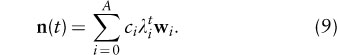
So as t becomes large, the solution will be determined by the largest-magnitude λi, termed the dominant eigenvalue and its eigenvector; hence,

where ≈ means approximately with a relative error decreasing to zero as t becomes large. This explains the numerical results (figure 1) that after an initial period of transients, the population grows at a constant rate, given by λ1, and the proportion of individuals in each age class becomes constant and is proportional to W1. For this reason w1 is called the stable age distribution.
The existence of a dominant eigenvalue is guaranteed so long as L is power positive: some power Lm has all entries greater than zero. L will be power positive providing fA > 0 and any two consecutive fs are positive, or more generally if all the entries of LA2+ 1 are positive. For a nonnegative L that is power positive, the Perron-Frobenius Theorem implies that L has a unique dominant eigenvalue that is real, positive, and strictly larger in magnitude than any other eigenvalue, guaranteeing convergence to the stable age distribution and stable growth rate λ1.
When the matrix lacks power positivity, we can get more exotic behavior. For example, consider a population where all the reproduction is concentrated in the last age class, such as

In this case, the age structure continually cycles with a cycle length of 3, and population size never settles into growing at a constant rate (figure 2). These population waves were initially explored by Harro Bernardelli in relation to oscillations in the age structure of the Burmese population. For a matrix like that in equation 11, with all reproduction in the final age class, each individual of age a at time t gives rise, after m time steps (where m is the number of age classes) to R0 age-a individuals at time t + m, and R0 is the product of the nonzero matrix entries. Consequently, any initial age structure gives rise to a cycle of age structures that repeats indefinitely with period A, and the long-term population growth rate is 
In a stage-structured model, individuals are divided into discrete categories conventionally called “stages” or “stage classes.” These sometimes represent discrete stages in the life history, say eggs, larvae, pupae, and adults of an insect species, but very commonly stages are categories imposed on a continuously varying trait such as size. For example, a plant population might be characterized by small, medium, and large individuals, and all between-stage transitions may be possible as a result of growth and shrinkage. Despite this, many of the ideas developed for age-structured populations carry over.
In place of the Leslie matrix, reproduction and the movements of surviving individuals between stages are governed by a population projection or Lefkovitch matrix, M. The dynamics are then given by

The Perron-Frobenius Theorem still applies provided that M is power positive, so the long-term growth rate is given by the dominant eigenvalue, λ1, of M, and the stable stage distribution by the corresponding eigenvector, w1.
To give a concrete example, here is the (slightly rounded) projection matrix used by Katriona Shea and David Kelly (1998) to explore the dynamics of Carduus nutans, an invasive thistle:

SB is the number of seeds in the seedbank, and S, M, L refer to thistle rosettes that are small, medium, and large in size. The matrix has the following simple interpretation: each column gives the expected contribution of a particular stage to each of the other stages. So the first column says that 4% of the seeds in the seedbank will stay there, and 19% will become small rosettes; the second column says that each small rosette will give rise to 8.25 seeds in the seedbank, 1.09 small rosettes, and a small number of medium and large rosettes, and so on.
Constructing the matrix M for a real population requires selecting appropriate stages. If the life cycle is divided into discrete stages, this is straightforward. Otherwise things become more complicated, as it is necessary to (1) decide on the appropriate measure of individual state and (2) set the boundaries between stages. Practical issues of data collection and the ability to predict an individual’s fate may determine how to measure an individual’s state. Typically a single variable is used (e.g., longest leaf length or rosette diameter as a measure of plant size), but more complex classifications, say by age and size, are also possible. Setting boundaries may be problematic. Ideally there should be many categories, so all individuals within a category really behave in a similar way, as the model assumes. However, the more categories there are, the fewer observations there are on each category, so estimates of the elements of M become less reliable. Integral projection models, discussed in the next section, provide an elegant way around these problems.
An enormous amount of work has been done analyzing the properties of projection matrices and using those properties to study real populations, much of it summarized in the landmark monograph by Hal Caswell (Caswell, 2001; first edition 1989). For example, we can use elasticity analysis to explore how fractional changes in matrix elements affect the long-term population growth rate λ1. Specifically, defining

Figure 2. Numerical solution of the Leslie matrix model (equation 11) assuming n(0) = (1, 1, 1) in each panel; we have a time series plot of (A) total population size N (t), (B) total population size averaged over the cycle, (C) the proportion of individuals in each age class (black = 0, dark gray = 1, and light gray = 2), and (D) the population growth rate N (t+1)/N (t)
it can be shown that

where v.w is the dot-product (v.w = v1w1 + v2w2 + … vnwn, and v is the left eigenvector of M (vM = λM). For the thistle matrix (equation 13), the elasticities are

These results suggest that the transitions SB → S, S → SB, and S → S are critical for population growth, and therefore, management strategies should focus on reducing these transitions. The unintuitive prediction that it will be far more effective to concentrate on small plants rather than large ones is made apparent only by computing the elasticities.
Matrix models can be generalized in many ways, such as by adding density dependence and/or stochastic variation from one time step to the next. Exploring all these would require an entire large book, which, fortunately, Caswell (2001) has already written.
Plant and many other types of organisms do not just come in small, medium, and large sizes. For example, consider Platte thistle, with individual size measured by the root crown diameter (figure 3). If individuals are divided into three size classes (indicated by the vertical lines in figure 3), then from the fitted curves, it is clear that some categories contain very different individuals; for example, individuals in the “large” category have probabilities of flowering that vary systematically from ≈0.2 to over 0.8. A matrix projection model with three size classes ignores these differences and treats all “large” individuals as identical.
To avoid this problem, in 2000 Michael R. Easterling, Stephen P. Ellner, and Philip M. Dixon proposed the integral projection model (IPM) in which individuals are characterized by a continuous variable x such as size. The state of the population given by n(x, t), such that the number of individuals with sizes between a and b is  n(x, t)dx. Instead of the matrix M, the IPM has a projection kernel K(y, x), so that
Figure 3. Size-structured demographic rates for Platte thistle, Cirsium canescens. (A) Growth (as characterized by plant size in successive years), (B) survival, (C) the probability of flowering, and (D) seed production all vary continuously with size and can be described by simple regression models. (Redrawn from Rose et al., 2005) In panels B and C, the data were divided into 20 equal-sized categories, and the plotted points are fractions within each category, but the logistic regression models (plotted as curves) were fitted to the binary values (e.g., flowering or not flowering) for each individual.

where s and S are the minimum and maximum possible sizes. The integration is the continuous version of equation 4, adding up all the contributions to size y at time t + 1 by individuals of size x at time t. Providing some technical conditions are met (see Ellner and Rees, 2006, for details), the IPM behaves essentially like a matrix model, and so the results described above carry over.
Constructing the projection kernel K(y, x) is straightforward using the regressions shown in figure 3. For an individual of size x to become size y, it must (1) grow from x to y, (2) survive, and (3) not flower (flowering is fatal in monocarpic plants like Platte thistle). These probabilities are calculated from the fitted relationships in figures 3A, 3B, and 3C, respectively. The use of regression models to construct the projection kernel brings some advantages: (1) accepted statistical approaches can be used for selecting an appropriate regression model; and (2) additional variables characterizing individuals’ states can be included by adding explanatory variables rather than having to select a single best state variable. For example, in some thistles the probability of flowering depends on both an individual’s size and age and is often described by a logistic regression such as logit pf (a, x) = exp (β0 + βs x + βaa). Extending a size-structured model to include age-dependent flowering therefore requires the estimation of a single additional parameter rather than estimation of many age- and size-class-specific flowering probabilities in the analogous matrix model.
The simplest starting point is the continuous-time analog of the Leslie matrix, in which vital rates depend only on individual age a, ignoring effects of population density and environmental factors. The state of the population (as usual counting only females) is then characterized by n(a, t), so that as in IPMs

The dynamics of n(a, t) are generated by the age-specific per capita birthrate b(a) and death rate μ(a). To be age a at time t, an individual must have been age a – dt at time t – dt and have not died; that is,

Rearranging and letting dt → 0, we obtain the McKendrick-von Foerster equation

which describes the dynamics of n(a, t) for a > 0. The boundary condition, describing the birth of new individuals, is
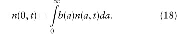
As with the previous models we expect exponential solutions, so n(a, t) ≈ Cn*(a)ert. By arguments analogous to those for the discrete-time age-structured model, the long-term instantaneous growth rate r can be shown to satisfy the continuous Euler-Lotka equation

where l(a) is the chance of surviving to age a given by

The fate of the population then depends on r, with increasing populations having r> 0 and decreasing ones r< 0. So not surprisingly r, like β, plays a key role in population management and life-history theory. Just as in the discrete case, we can compute expected lifetime fecundity

so r > 0 if and only if R0 > 1, as expected.
Age has the unforgiving property that one year on, you will always be one year older, and this property was exploited when studying age-structured models. In a size-structured model, we must specify how size changes over time. It is then possible, by looking at the flows of individuals into and out of some small size range, to derive the dynamics of the size structure. If individuals grow deterministically, growth can be described by an equation dm/dt = g(m). This leads to the McKendrick-von Foerster equation for size-structured dynamics (although it was almost surely known to Euler as the equation for passive particles carried by a moving fluid):

Specifying appropriate boundary conditions is less straightforward for equation 20 than for equation 17. If we assume that individuals are size m0 at birth, then equation 20 applies for m > m0, and the boundary condition is

the prefactor before the integral is needed to convert the birthrate (individuals per unit time) into the resulting contribution to the size distribution (individuals per increment of size). Much as for age-structured models, the size-structured model has a long-term size structure and population growth rate, which can be derived using the (nonlinear) relationship between age and size entailed by the deterministic growth pattern. The basic model can be extended in many ways, such as allowing a random component to growth (including a chance of shrinkage), variable offspring size, reproduction by fission, and characterization of individuals by multiple measures of size (e.g., lipid and nonlipid body mass) or by size and age.
Extending the basic models to include density dependence and interspecific interactions is difficult, and indeed, William S. C. Gurney and Roger Nisbet (1998) described continuous-time models in which individuals are distinguishable by age and size as “a traditional source of mathematical headaches.” To make some progress, Gurney, Nisbet, and John Lawton (1983) suggested grouping individuals into stages and assuming constant vital rates within each stage. However, unlike the stage-structured matrix model, individuals within a stage may have different states. For example, even if all juveniles have the same growth rate, younger juveniles may be smaller and less likely to mature soon into adults.
To see what this means, consider Gurney, Nisbet, and Lawton’s model for laboratory blowfly populations based on the classic experimental studies of A. J. Nicholson. The model assumes two stages, Juvenile and Adult.
These assumptions imply a set of differential equations describing the dynamics,

where RJ(t) and RA(t) are the recruitment rates into the Juvenile and Adult stages. By definition, Rj(t)  . Because the Juvenile stage lasts exactly τ time units, RA(t) equals the recruitment into the Juvenile stage t — τ time units ago times the survival through the Juvenile stage SJ= e–τμJ; hence, RA(t) = SJRJ(t — τ). Substituting Rj(t) into RA(t) gives a single equation for the dynamics

The key simplifying assumption in this model is that all Juveniles have the same demographic rates. Juveniles do differ in their state though: some are nearly mature and will soon become adults, whereas others are recently born and will not become mature for some time. Although the final model involves only the total numbers in each class, its structure reflects the fact that newborns all wait τ time units before maturing into Adults. The presence of the time delay τ is the price for allowing individuals within a stage to differ in state. In this model, stages correspond exactly to a range of ages, but similar models can be constructed in which stages correspond to a range of sizes, or in which there is no exact correspondence of stages to age or size; rather, each individual within a stage has a probability (potentially depending on age, size, etc.) of making the transition to another stage. These models may require state variables in addition to the population counts for each stage to track the within-stage state dynamics and its consequences.
Here we discuss some applications of the ideas presented in the previous sections: a stochastic densitydependent Leslie matrix model for an Asiatic wild ass; stage-structured models used to understand the dynamics of laboratory populations; and use of integral projection models to make evolutionary predictions of life-history strategies.
David Saltz, Daniel I. Rubinstein, and Gary C. White (2006) developed a Leslie matrix-type model for the population of an Asiatic wild ass (Equus hemionus) reintroduced into the Makhtesh Ramon Nature Reserve in Israel, based on long-term monitoring (1985–1999). Their main goal was to explore possible effects of increased rainfall variability on the population’s risk of extinction because increased variability is predicted under some global climate change scenarios even in areas where no changes in mean rainfall are predicted.
Their model includes a number of important extensions to the basic Leslie matrix model described above. Saltz et al. used their data to fit a model predicting an adult (age ≥ 3) female’s chance of successful reproduction as a function of total rainfall in the current and previous years. Their model also included a negative effect of adult female density, but reproductive success was unrelated to age. Age-specific survivorship was based on a published survivorship curve for zebra, with additional mortality of 30% or higher during drought years (rainfall < 40 mm) based on data for other ungulates.
Figure 4. Probabilities of extinction of an Asiatic wild ass population under various climate change scenarios.
Because the model was explicitly linked to variation in rainfall, model simulations could be based on the 41 years of rainfall data for the study area. In particular, simulations to assess extinction risk over a 100-year time period were run by bootstrapping from either the first 20 years of rainfall data (when variance was lower), the second 21 years (when variance was higher), or the complete data set. They also incorporated demographic stochasticity: for example, rather than having 30% of adults die in a drought year, they did a simulated “coin toss” to determine whether each individual lived or died.
The strong effect of drought years on survival and reproduction produced a strong impact of rainfall variability on population persistence. At the low-end estimate of drought-induced mortality (30%), the increase in variance between the first and second halves of the rainfall data produced a more then fivefold increase in the probability of population extinction within 100 years (figure 4).
Gurney et al. (1983) used Nicholson’s data to estimate the parameters for the model in equation 23. Nicholson conducted a series of long-term experiments, using sheep blowflies, designed to explore the effects of resource limitation at different life stages. The blowfly has four distinct life stages—eggs, larvae, pupae, and adults—but feeds only in the larval and adult stages. In the experiments considered by Gurney et al., larvae were given unlimited resources, whereas the adults received protein (in the form of ground liver) at a fixed rate, leading to competition. To apply the stage-structured model, Gurney et al. (1983) estimated the stage-specific mortalities, fecundities, and durations:
With these estimates, the model produces sustained cycles with a period of about 37 days (compared to an average observed period of about 38 days), and adult population varying between a minimum of 150 and a maximum of 5400 (compared to observed minima and maxima of 270 ± 120 and 7500 ± 500; figure 5). This is remarkable given that no model parameters were adjusted to fit the experimental time series, and perhaps even more remarkably the model solutions exhibit the “double peak” that usually occurred in the data. The population cycles occur because egg production is overcompensating, and the period of the cycles is determined by τ; analysis of the model suggests the period will be in the range (2τ,4τ), in good agreement with the numerical solution.
To simulate the model without the difficulties of solving delay-differential equations, it can be expressed as an age-structured model, similar to equation 2. Because the maturation time is 15.6 days, it is convenient to use time and age increments of 0.1 days. The instantaneous mortality and fecundity rates in the continuous-time model can be converted into rates per 0.1 days. For example, if juveniles in the discrete-time model become mature adults when they exit the 15.6-day-old age class, the juvenile survival probability in the discrete-time model is  per time increment. Then 157 age classes are needed for the juveniles, but only one for the adults, giving a Leslie matrix that is large (of size 158û158) and density dependent but straightforward to implement on a computer.
Population dynamics and evolution are intimately linked because the fate of new genetic mutants depends on their ability to spread in a population. Coupling evolutionary ideas with demographic models for the growth of the mutant subpopulation thus allows predictions of how natural selection shapes individual behaviors and life histories. The key evolutionary idea is John Maynard Smith’s concept of an evolutionary stable strategy (ESS): a strategy that cannot be displaced by a rare mutant if it has become fixed in a population. In a population at demographic equilibrium (λ= 1), the established strategy cannot be displaced if λ is less than 1 for a rare mutant strategy with some other strategy. In this way, ESSs in real populations can be identified.
Figure 5. (A) Experimental time series of blowfly adult (gray) and egg (black) dynamics (from Nicholson, 1954) and (B) predicted dynamics from the simple stage-structured model (equation 23).
As an illustration, an integral projection model for Oenothera biennis (evening primrose) can be used to predict the size dependence of flowering probability (figure 3C). This relationship is determined by balancing the benefits of flowering at a large size (increased seed production, figure 3D) against the mortality costs of growing large. Using published data, Rees and Rose (2002) produced a fully parameterized IPM for this species. The probability of flowering was size dependent and described by a logistic regression, logitpf (x) = β0 + βsx, where x is log rosette diameter, β0 and βs and the fitted intercept and slope. Making β0 smaller reduces the probability of flowering for all sizes and so increases the mean size at flowering. In Oenothera, density dependence acts only at the recruitment stage, so the ESS is characterized by maximizing R0, the total reproductive output of an individual that survives through the recruitment stage (Mylius and Diekmann, 1995). Numerical evaluation of R0 as a function of β0 shows that estimated value is very close to the predicted ESS (figure 6). This example illustrates how structured population models, coupled with evolutionary ideas, provide a general framework for understanding the evolution of organisms’ life cycles subject to trade-offs and constraints, a vast subject known as life-history theory.
All populations are structured: by age, size, genotype, social status, and so on. Structured population models have arguably become the core theoretical framework for population ecology, and a modern course on population ecology would be in large part a course on structured population modeling. The scope of theory and applications vastly exceeds the space available here. Read on!
Figure 6. Relationships between β0 and (A) R0 and (B) λ for the Oenothera IPM. The ESS is marked with a dot, and the estimated β0 is indicated by the vertical line.
Caswell, Hal. 2001, Matrix Population Models: Construction, Analysis and Interpretation. Sunderland, MA: Sinauer Associates (1st edition 1989). This volume is the classic and comprehensive monograph on matrix models for structured populations, clear, authoritative, and amusing. This book and the ones below by Metz and Diekmann, Tuljapurkar, and Tuljapurkar and Caswell are essential reading for the structured population modeler.
Ellner, Stephen P., and Mark Rees. 2006. Integral projection models for species with complex demography. American Naturalist 167: 410–428. This article generalized the sizestructured IPM introduced by Easterling, Ellner, and Dixon by allowing individuals to be cross-classified by several traits. The article includes model construction, elasticity analysis, stable distribution theory for densityindependent models, evolutionary optimality criteria, and local stability analysis for density-dependent models.
Gurney, William S. C., and Roger M. Nisbet. 1998. Ecological Dynamics. Oxford: Oxford University Press. This volume is a very readable text covering a wide range of structured population models, with many case studies that illustrate the concepts and processes involved in constructing structured models.
Gurney, W.S.C., R. M. Nisbet, and John. H. Lawton. 1983. The systematic formulation of tractable single-species population models incorporating age structure. Journal of Animal Ecology 52: 479–495. This paper introduced continuous-time models with discrete stage structure and showed how they could explain qualitative differences between the dynamics of two laboratory insect populations.
Metz, Johannes A. J., and Odo Diekmann, eds. 1986. The Dynamics of Physiologically Structured Populations. Berlin: Springer. This is the volume that moved continuoustime size-structured models and their relatives into the mainstream of population modeling, with a mix of mathematical theory and applications. Often mathematically challenging; the article by de Roos in Tuljapurkar and Caswell (1997) provides a “gentle introduction” that may be useful to read first.
Murdoch, William M., Cheryl J. Briggs, and Roger M. Nisbet. 2003. Consumer-Resource Dynamics. Princeton, NJ: Princeton University Press. This definitive volume presents systematic development and real-world applications of stage-structured models in the style of Gurney-Nisbet-Lawton for predator-prey and host-parasitoid population interactions, summarizing the fruits from two decades of focused effort. If we could all work like this, ecology would be much the better for it.
Mylius, Sido D., and Odo Diekmann. 1995. On evolutionarily stable life-histories, optimization and the need to be specific about density-dependence. Oikos 74: 218–224. This represents an elegant theoretical paper analyzing the properties that characterize ESSs in structured populations.
Tuljapurkar, Shripad. 1990. Population Dynamics in Variable Environments. New York: Springer. Although sadly now out of print, this volume is an essential reference on stochastic matrix models by the author of many fundamental articles on this topic.
Tuljapurkar, S., and H. Caswell, eds. 1997. Structured-Population Models in Marine, Terrestrial, and Freshwater Systems. New York: Chapman & Hall. This book provides a wealth of applications, and some accessible reviews of basic theory, derived from a summer course on structured population models at Cornell University.
Rees, M., and K. E. Rose. 2002. Evolution of flowering strategies in Oenothera glazioviana: An integral projection model approach. Proceedings of the Royal Society 269: 1509–1515.
Rose, K. E., S. M. Louda, and M. Rees. 2005. Demographic and evolutionary impacts of native and invasive insect herbivores: A case study with Platte thistle, Cirsium canescens. Ecology 86: 453–465.
Saltz, David, Daniel I. Rubenstein, and Gary C. White. 2006. The impact of increased environmental stochasticity due to climate change on the dynamics of Asiatic wild ass. Conservation Biology 20: 1402–1409.
Shea, K., and D. Kelly. 1998. Estimating biocontrol agent impact with matrix models: Carduus nutans in New Zealand. Ecological Applications 8: 824–832.


