1. Metapopulation patterns and processes
2. Long-term viability of metapopulations
3. Metapopulations in changing environments
4. Evolution in metapopulations
5. Spatial dynamics in nonpatchy environments
6. Metapopulations, spatial population processes, and conservation
Most landscapes are complex mosaics of many kinds of habitat. From the viewpoint of a particular species, only some habitat types, often called “suitable habitat,” provide the necessary resources for population growth. The remaining landscape, often called the (landscape) matrix, can only be traversed by dispersing individuals. Often the suitable habitat occurs in discrete patches, an example of which is a woodland in the midst of cultivated fields—for forest species, the woodland is like an island in the sea. The woodland may be occupied by a local population of a forest species, but many such patches are likely to be temporarily unoccupied because the population became extinct in the past and a new one has not yet been established. At the landscape level, woodlands and other comparable habitat patches comprise networks in which local populations living in individual patches are connected to each other by dispersing individuals. A set of local populations inhabiting a patch network is called a metapopulation. In other cases, the habitat does not consist of discrete patches, but even then, habitat quality is likely to vary from one place to another. Habitat heterogeneity tends to be reflected in a more or less fragmented population structure, and such spatially structured populations may be called metapopulations. Metapopulation biology addresses the ecological, genetic, and evolutionary processes that occur in metapopulations. For instance, in a highly fragmented landscape, all local populations may be so small that they all have a high risk of extinction, yet the metapopulation may persist if new local populations are established by dispersing individuals fast enough to compensate for extinctions. Metapopulation structure and the extinction–colonization dynamics may greatly influence the maintenance of genetic diversity and the course of evolutionary changes. Metapopulation processes play a role in the dynamics of most species because most landscapes are spatially more or less heterogeneous, and many comprise networks of discrete habitat patches. Human land use tends to increase fragmentation of natural habitats, and hence, metapopulation processes are particularly consequential in many human-dominated landscapes.
connectivity. An individual habitat patch in a patch network and a local population in a metapopulation are linked to other local populations, if any exist, via dispersal of individuals. Connectivity measures the expected rate of dispersal to a particular patch or population from the surrounding populations.
dispersal. Movement of individuals among local populations in a metapopulation is dispersal. Migration is often used as a synonym of dispersal.
extinction–colonization dynamics. Local populations in a metapopulation may go extinct for many reasons, especially when the populations are small. New local populations may become established in currently unoccupied habitat patches. Local extinction and recolonization are called turnover events.
extinction debt. If the environment becomes less favorable for the persistence of metapopulations through, e.g., habitat loss and fragmentation, species’ metapopulations start to decline. For some metapopulations, the new environment may be below the extinction threshold. Extinction debt is defined as the number of species for which the extinction threshold is not met and that are therefore predicted to become extinct but have not yet had time to become extinct.
extinction threshold. Classic metapopulation may persist in a habitat patch network in spite of local extinctions if the rate of recolonization is sufficiently high. Long-term persistence is less likely the smaller the habitat patches are (leads to high extinction rate) and the lower their connectivity (leads to low recolonization rate). Below extinction threshold, recolonizations do not occur fast enough to compensate for local extinctions, and the entire metapopulation becomes extinct even if some habitat patches exist in the landscape.
local population. This is an assemblage of individuals sharing common environment, competing for the same resources, and reproducing with each other. In a fragmented landscape, a local population typically inhabits a discrete habitat patch.
metapopulation. A classic metapopulation is an assemblage of local populations living in a network of habitat patches. More generally, spatially structured populations at landscape scales are often called metapopulations.
metapopulation capacity. This is a measure of the size of the habitat patch network that takes into account the total amount of habitat as well as the influence of fragmentation on metapopulation viability.
network of habitat patches. In a fragmented landscape, habitat occurs in discrete patches, each one of which may be occupied by a local population, and which together compose a network that may be occupied by a metapopulation.
source and sink populations and habitats. A local population that has negative expected growth rate, and that therefore would go extinct without immigration, is called a sink population, and the respective habitat is a sink habitat. A population that has sufficiently high growth rate when small to persist even without immigration is called a source population, and the respective habitat is source habitat.
Many classifications of metapopulations have been proposed, and they serve a purpose in facilitating communication, but it should be recognized that in reality there exists a continuum of spatial population structures rather than discrete types. The following terms are often used.
Classic metapopulations consist of many small or relatively small local populations in patch networks. Small local populations have high or relatively high risk of extinction, and hence, long-term persistence can occur only at the metapopulation level, in a balance between local extinctions and recolonizations (further discussed under the Levins Model below).
Mainland–island metapopulations include one or more populations that are so large and live in sufficiently big expanses of habitat that they have a negligible risk of extinction. These populations, called mainland populations, are stable sources of dispersers to other populations in smaller habitat patches (island populations). The MacArthur-Wilson model of island biogeography is an extension of the mainland–island metapopulation model to a community of many independent species.
Source–sink metapopulations include local populations that inhabit low-quality habitat patches and would therefore have negative growth rate in the absence of immigration (sink populations), and local populations inhabiting high-quality patches in which the respective populations have positive growth rates (source populations; further discussed under Source and Sink Populations below).
Nonequilibrium metapopulations are similar to classic metapopulations, but there is no stochastic balance between extinctions and recolonizations, typically because the environment has recently changed and the extinction rate has increased, the recolonization rate has decreased, or both (this is further discussed under Transient Dynamics and Extinction Debt below).
Three ecological processes are fundamental to metapopulation dynamics: dispersal, colonization of currently unoccupied habitat patches, and local extinction. Dispersal has several components: emigration, departure of individuals from their current population; movement through the landscape; and immigration, arrival at new populations or at empty habitat patches. All three components depend on the traits of the species and on the characteristics of the habitat and the landscape, but they may also depend on the state of the population, for instance, on population density.
Dispersal may influence local population dynamics. In the case of very small populations, a high rate of emigration may reduce population size and thereby increase the risk of extinction. Conversely, immigration may enhance population size sufficiently to reduce the risk of extinction. Immigration to a currently unoccupied habitat patch is particularly significant in potentially leading to the establishment of a new local population. From the genetic viewpoint, two extreme forms of immigration and gene flow have been distinguished, the “migrant pool” model, in which the dispersers are drawn randomly from the metapopulation, and the “propagule pool” model, in which all immigrants to a patch originate from the same source population. The latter is likely to reduce genetic variation in the metapopulation.
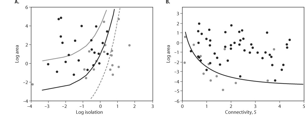
Figure 1. Two examples of the common metapopulation pattern of increasing incidence (probability) of habitat patch occupancy with increasing patch area and connectivity. Black circles represent occupied, gray circles unoccupied, habitat patches at the time of sampling. (A) Mainland–island metapopulation of the shrew Sorex cinereus on islands in North America. Isolation, which increases with decreasing connectivity, is here measured by distance to the mainland. The lines indicate the combinations of area and isolation for which the predicted incidence of occupancy is greater than 0.1, 0.5, and 0.9, respectively. (From Hanski, I. 1993. Dynamics of small mammals on islands. Ecography 16: 372–375) (B) Classic metapopulation of the silver-spotted skipper butterfly (Hesperia comma) on dry meadows in southern England. The line indicates the combinations of area and connectivity above which the predicted incidence of occupancy is greater than 0.5. (From Hanski, I. 1994. A practical model of metapopulation dynamics. Journal of Animal Ecology 63: 151–162)
Colonization of a currently unoccupied habitat patch is more likely the greater the numbers of immigrants, which is measured by the connectivity of the patch (see next section). All populations have smaller or greater risks of extinction from demographic and environmental stochasticities (see Stochasticity in Metapopulation Dynamics below) and other causes. Typically, the smaller the population the greater the risk of extinction.
Assuming that a local population in patch i has a constant risk of going extinct, Ei, and that patch i, if unoccupied, has a constant probability of becoming recolonized, Ci, the state of patch i, whether occupied or not, is determined by a stochastic process (Markov chain) with the stationary (time-invariant) probability of occupancy given by
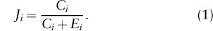
Ji is often called the incidence of occupancy. This formula helps explain the common metapopulation patterns of increasing probability of patch occupancy with patch area (which typically decreases Ei and hence increases Ji) and with decreasing isolation (which typically increases Ci and hence increases Ji). Figure 1 gives two examples.
Local populations and habitat patches in a patch network are linked via dispersal. Connectivity measures the strength of this coupling from the viewpoint of a particular patch or local population. Connectivity is best defined as the expected number of individuals arriving per unit time at the focal patch. Connectivity increases with the number of populations (sources of dispersers) in the neighborhood of the focal patch; with decreasing distances to the source populations (making successful dispersal more likely); and with increasing sizes of the source populations (larger populations send out more dispersers). A measure of connectivity for patch i that takes all these factors into account may be defined as
Table 1. Four types of stochasticity affecting metapopulation dynamics
| Type of stochasticity | Entity affected | Correlation among entities |
| Demographic | Individuals in local populations | No |
| Environmental | Individuals in local populations | Yes |
| Extinction–colonization | Populations in metapopulations | No |
| Regional | Populations in metapopulations | Yes |
Here, Aj is the area and Jj is the incidence of occupancy of patch j, dij is the distance between patches i and j, 1/α is species-specific average dispersal distance, and ζim and ζem describe the scaling of immigration and emigration with patch area. This formula assumes that the sizes of source populations are proportional to the respective patch areas; if information on the actual population sizes Nj is available, the surrogate Jj Aj in equation 2 may be replaced by Nj.
Metapopulation dynamics are influenced by four kinds of stochasticity (types of random events; table 1): demographic and environmental stochasticity affect each local population, and extinction–colonization and regional stochasticity affect the entire metapopulation. Both local dynamics and metapopulation dynamics are inherently stochastic because births and deaths in local populations are random events (leading to demographic stochasticity) and so are population extinctions and recolonizations in a metapopulation (extinction–colonization stochasticity). Environmental stochasticity refers to correlated temporal variation in birth and death rates among individuals in local populations, whereas regional stochasticity refers to correlated extinction and colonization events in meta-populations. Metapopulations are typically affected by regional stochasticity because the processes generating environmental stochasticity, including temporally varying weather conditions, are typically spatially correlated.
It can be demonstrated mathematically that all metapopulations with population turnover caused by extinctions and colonizations will eventually become extinct. It is a certainty that, given enough time, a sufficiently long run of extinctions will arise by “bad luck” and extirpate the metapopulation. However, time to extinction can be very long for large meta-populations inhabiting large patch networks (see the Levins Model below), and the metapopulation settles for a long time to a stochastic quasiequilibrium, in which there is variation but no systematic change in the number of local populations.
Populations may occur in low-quality sink habitats if there is sufficient dispersal from other populations living in high-quality source habitats. Therefore, the presence of a species in a particular habitat patch does not suffice to demonstrate that the habitat is of sufficient quality to support a viable population. Conversely, a local population may be absent from a habitat patch that is perfectly suitable for population growth when a local population happened to become extinct for reasons unrelated to habitat quality.
In a temporally varying environment, sink populations may, counterintuitively, enhance metapopulation persistence. This may happen when source populations exhibit large fluctuations leading to a high risk of extinction. The habitat patches supporting such sources may become recolonized by dispersal from sinks, assuming this happens before the sink populations have declined to extinction. In general, dispersal among local populations that fluctuate relatively independently of each other (weak regional stochasticity) enhances the metapopulation growth rate. This happens because when a population has increased in size in a good year, and the offspring are spread among many independently fluctuating populations, subsequent bad years will not hit them all simultaneously. It can be shown that this spreading-of-risk effect of dispersal may be so substantial that it allows a metapopulation consisting of sink populations only to persist without any sources.
Mathematical models are used to describe, analyze, and predict the dynamics of metapopulations living in fragmented landscapes. A wide range of models can be constructed differing in the forms of stochasticity they include (see Stochasticity in Metapopulation Dynamics above), in whether change in metapopulation size occurs continuously or in discrete time intervals, in how many local populations the metapopulation consists of, in how the structure of the landscape is represented, and so forth. A minimal metapopulation includes two local populations connected by dispersal. At the other extreme, assuming infinitely many habitat patches leads to a particularly simple description of the classic metapopulation, which is discussed next.
The Levins model has special significance for metapopulation ecology, as it was with this model that the American biologist Richard Levins introduced the metapopulation concept in 1969. The Levins model captures the essence of the classic metapopulation concept—that a species may persist in a balance between stochastic local extinctions and recolonization of currently unoccupied patches. For mathematical convenience, the model assumes an infinitely large network of identical patches, which have two possible states, occupied or empty. The state of the entire metapopulation can be described by the fraction of currently occupied patches, p, which varies between 0 and 1.
If each local population has the same risk of extinction, and each population contributes equally to the rate of recolonization, the rate of change in the size of the metapopulation is given by
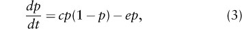
where c and e are colonization and extinction rate parameters. This model ignores stochasticity, but it is a good approximation of the corresponding stochastic model for a large metapopulation inhabiting a large patch network. The Levins model is structurally identical with the logistic model of population growth, which can be seen by rewriting equation 3 as
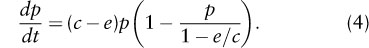
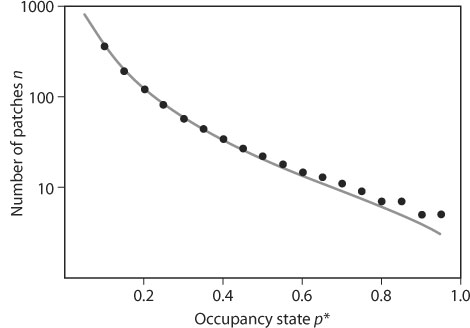
c – e gives the rate of metapopulation growth when it is small, and 1 – e/c is the equilibrium metapopulation size (“carrying capacity”). The ratio c/e defines the basic reproductive number R0 in the Levins model. A species can increase in a patch network from low occupancy if R0 = c/e > 1. This condition defines the extinction threshold in metapopulation dynamics. In reality, in a finite patch network, a metapopulation may become extinct because of stochasticity even if the threshold condition c/e > 1 is satisfied. When a diffusion approximation is used to analyze the stochastic Levins model, the mean time to extinction T can be calculated as a function of the number of habitat patches n and p*, the size of the metapopulation at quasiequilibrium. Figure 2 shows the number of patches that the network must have to make T at least 100 times as long as the expected lifetime of a single local population (given by the inverse of the extinction rate). For metapopulations with large p*, a modest network of n = 10 patches is sufficient to allow long-term persistence, but for rare species (say p* < 0.2), a large network of n > 100 is needed for long-term persistence.
Figure 2. The number of habitat patches n needed to make the mean time to metapopulation extinction T at least 100 times longer than the mean time to local extinction. The dots show the exact result based on the stochastic logistic model, and the line is based on the following diffusion approximation:
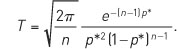
(From Ovaskainen and Hanski, 2003)
The stochastic Levins model includes extinction–colonization stochasticity but no regional stochasticity, which leads to correlated extinctions and colonizations. In the presence of regional stochasticity, the mean time to metapopulation extinction does not increase exponentially with increasing n as in figure 2 but as a power function of n, the power decreasing with increasing correlation in extinction and recolonization rates, reducing long-term viability. This result is analogous to the well-known effects of demographic and environmental stochasticities on the lifetime of single populations.
There is no description of landscape structure in the Levins model; hence, it is not possible to investigate with this model the consequences of habitat loss and fragmentation. Real metapopulations live in patch networks with a finite number of patches; the patches are of varying size and quality, and different patches have different connectivities, which affect the rates of immigration and recolonization. These considerations have been incorporated into spatially realistic metapopulation models. The key idea is to model the effects of habitat patch area, quality, and connectivity on the processes of local extinction and recolonization. Generally, the extinction risk decreases with increasing patch area because large patches tend to have large populations with a small risk of extinction, and the colonization rate increases with connectivity to existing populations.
The theory provides a measure to describe the capacity of an entire patch network to support a metapopulation, denoted by λM and called the metapopulation capacity of the fragmented landscape. Mathematically, λM is the leading eigenvalue of a landscape” matrix, which is constructed with assumptions about how habitat patch areas and connectivities influence extinctions and recolonizations. The size of the metapopulation at equilibrium is given by

which is similar to the equilibrium in the Levins model, but with the difference that metapopulation equilibrium now depends on metapopulation capacity, and metapopulation size pλ is measured by a weighted average of patch occupancy probabilities. The threshold condition for metapopulation persistence is given by

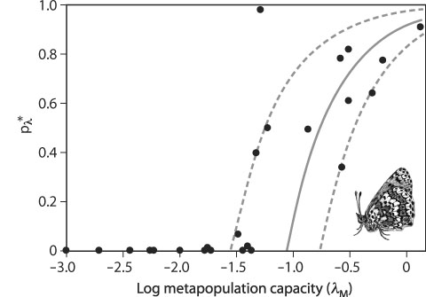
In words, metapopulation capacity has to exceed a threshold value, which is set by the extinction proneness (e) and colonization capacity (c) of the species, for long-term persistence. To compute λM for a particular landscape, one needs to know the range of dispersal of the focal species, which sets the spatial scale for calculating connectivity (parameter α in equation 2), and the areas and spatial locations of the habitat patches. The metapopulation capacity can be used to rank different fragmented landscapes in terms of their capacity to support a viable metapopulation: the larger the value of λM, the better the landscape. Figure 3 gives an example in which metapopulation capacity explains well the size of butterfly metapopulations in dissimilar patch networks.
A fundamental question about metapopulation dynamics concerns long-term viability, which has great significance for the conservation of biodiversity in fragmented landscapes (see Metapopulations, Spatial Population Processes, and Conservation below). A patch network will not support a viable metapopulation unless the extinction threshold is exceeded, and even if it is, a metapopulation may become extinct for stochastic reasons (see Levins Model above). Long-term viability is further reduced by environmental change.
Figure 3. Metapopulation size of the Glanville fritillary butterfly (Melitaea cinxia) as a function of the metapopulation capacity λM in 25 habitat patch networks. The vertical axis shows the size of the metapopulation based on a survey of habitat patch occupancy in 1 year. The empirical data have been fitted by a spatially realistic model (continuous line; the broken lines give the model fit to the second smallest and the second largest positive values). The result provides a clear-cut example of the extinction threshold. (From Hanski and Ovaskainen, 2000)
Innumerable species of fungi, plants, and animals live in ephemeral habitats such as decaying wood. A dead tree trunk may be viewed as a habitat patch for local populations of such organisms. The trunk is not permanent, largely because of the action of the organisms themselves, and local populations necessarily become extinct at some point. Parasites living in a host individual can be similarly considered as comprising a local population, which necessarily becomes extinct when the host individual dies. This example reflects fundamental similarities between metapopulation biology and epidemiology.
Regular disappearance of habitat patches increases extinctions, but the metapopulation may still persist in a stochastic quasiequilibrium. Equation 1 may be extended to include patch extinction and the appearance of new patches:
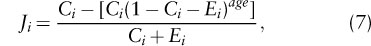
where age is the age of patch i. Following its appearance, a new patch is initially unoccupied, Ji = 0 when age = 0. When the patch becomes older, the incidence of occupancy approaches the equilibrium [Ci (Ci + Ei)] given by equation 1 and determined by the extinction–colonization dynamics of the species. The precise trajectory is given by equation 7, where the term in square brackets declines from Ci when age = 0 to zero as age becomes large and when equation 1 is recovered.
Human land use often causes the loss and fragmentation of the habitat for many other species. Following the change in landscape structure, especially if the change is abrupt, it takes some time before the metapopulation has reached the new quasiequilibrium, which may be metapopulation extinction. Considering a community of species, the term extinction debt refers to situations in which, following habitat loss and fragmentation, the threshold condition is not met for some species, but these species have not yet become extinct because they respond relatively slowly to environmental change. More precisely, the extinction debt is the number of extant species that are predicted to become extinct, sooner or later, because the threshold condition for long-term persistence is not satisfied for them following habitat loss and fragmentation.
How long does it take before the metapopulation has reached the new quasiequilibrium following a change in the environment? The length of the transient period is longer when the change in landscape structure is greater, when the rates of extinction and recolonization are lower, and when the new quasiequilibrium following environmental change is located close to the extinction threshold. The latter result has important implications for conservation. Species that have become endangered as a result of recent changes in landscape structure are located, by definition, close to their extinction threshold, and hence, the transient period in their response to environmental change is predicted to be long. This means that we are likely to underestimate the level of threat to endangered species because many of them do not occur presently at quasiequilibrium with respect to the current landscape structure but are slowly declining because of past habitat loss and fragmentation. On the positive side, long transient time in metapopulation dynamics following environmental change gives us humans more time to do something to reverse the trend.
The hierarchical structure of metapopulations, from individuals to local populations to the entire metapopulation, has implications for evolutionary dynamics. In addition to natural selection occurring within local populations, different selection pressures may influence the fitness of individuals during dispersal and at colonization. Individuals that disperse from their natal population and succeed in establishing new local populations are likely to comprise a nonrandom group of all individuals in the metapopulation. Particular phenotypes and genotypes may persist in the metapopulation because of their superior performance in dispersal and colonization even if they would be selected against within local populations. This is often called the metapopulation effect.
The most obvious example relates to emigration rate and dispersal capacity. The most dispersive individuals are selected against locally because their local reproductive success is reduced by early departure. However, these individuals may find a favorable habitat elsewhere, which increases their fitness in the metapopulation. Which particular phenotypes and genotypes are favored in particular metapopulations depends on many factors. Local competition for resources and competition with relatives for mating opportunities selects for more dispersal, and so does temporal variation in fitness among populations, but mortality during dispersal selects against dispersal. Because of many opposing selection pressures, habitat fragmentation may select for more or less dispersive individuals depending on particular circumstances.
The classic population concept and corresponding population models assume that all individuals interact equally with all other individuals in the population. This is called panmictic population structure. On the other extreme is the classic metapopulation concept, which assumes a set of dynamically independent local populations, within which individual interactions take place. Many real populations have intermediate spatial population structures: individuals do not occur in discrete local populations, but the population is more continuous across a large area, yet ecological interactions and dispersal are more or less localized; hence, the population is not panmictic at a large spatial scale. In this case, what matters most is the local density experienced by individuals rather than the overall density of individuals in the large population as a whole.
Population dynamics across a landscape is determined by the opposing forces of localized interactions, which tend to increase differences in local dynamics and dispersal among neighboring population units, which reduces their dynamic independence. In single panmictic populations, strongly nonlinear dynamics may lead to population cycles and other complex dynamics. In large populations distributed across a landscape, nonlinear dynamics and dispersal may generate complex spatially structured dynamics. For instance, the dynamics of measles in human populations may exhibit traveling waves, in which epidemics initiated in large core populations (cities) lead, with some time lag, to epidemics in the surrounding smaller communities (see chapter II.9). Comparable complex spatiotemporal patterns of population density have been detected in some animal populations.
Loss and fragmentation of natural habitats are the most important reasons for the current catastrophically high rate of loss of biodiversity on Earth. The amount of habitat matters because long-term viability of populations and metapopulations depends, among other things, on the environmental carrying capacity, which is typically positively related to the total amount of habitat. Additionally, the spatial configuration of habitat may influence viability because most species have limited dispersal range, and hence, not all habitat in a highly fragmented landscape is readily accessible, giving rise to the extinction threshold (see Levins Model above).
Metapopulation models have been used to address the population dynamic consequences of habitat loss and fragmentation. In the Levins model, where there is no description of landscape structure, habitat loss has been modeled by assuming that a fraction 1 – h of the patches becomes unsuitable for reproduction, while fraction h remains suitable. Such habitat loss reduces the colonization rate to cp(h – p). The species persists in a patch network if h exceeds the threshold value e/c. At equilibrium, the fraction of suitable but unoccupied patches (h – p*) is constant and equals the amount of habitat at the extinction threshold (h = e/c).
The spatially realistic metapopulation model (see above) combines the metapopulation perspective of the Levins model with a description of the spatial distribution of habitat in a fragmented landscape. In the model described by equation 5, the metapopulation capacity λM replaces the fraction of suitable patches h in the Levins model, and the threshold condition for metapopulation persistence is given by λM > e/c. λM takes into account not only the amount of habitat in the landscape but also how the remaining habitat is distributed among the individual habitat patches and how the spatial configuration of habitat influences extinction and recolonization rates and hence metapopulation viability. The metapopulation capacity can be computed for multiple landscapes, and their relative capacities to support viable metapopulations can be compared: the greater the value of λM, the more favorable the landscape is for the particular species (figure 3).
Setting aside a sufficient amount of habitat as reserves is essential for conservation of biodiversity. Reserve selection should be made in such a manner that a given amount of resources for conservation makes a maximal contribution toward maintaining biodiversity. In the past, making the optimal selection of reserves out of a larger number of potential reserves was typically based on their current species richness and composition, without any consideration for the long-term viability of the species in the reserves. More appropriately, we should ask which selection of reserves maintains the largest number of species to the future, taking into account the temporal and spatial dynamics of the species and the predicted changes in climate and land use. Metapopulation models can be incorporated into analyses that aim at providing answers to such questions.
Metapopulations are assemblages of local populations inhabiting networks of habitat patches in fragmented landscapes. The local populations have more or less independent dynamics because of their isolation, but complete independence is prevented by large-scale similarity in environmental conditions and by dispersal, which occurs at a spatial scale characteristic for each species. Metapopulation models are used to describe, analyze, and predict the dynamics of metapopulations. Important questions include the conditions under which metapopulations may persist in particular patch networks and for how long, how landscape structure influences metapopulation persistence, and the response of metapopulations to changing landscape structure. Metapopulation dynamics in highly fragmented landscapes involves an extinction threshold, a critical amount, and spatial configuration of habitat that is necessary for long-term persistence of the metapopulation.
Hanski, I. 1999. Metapopulation Ecology. Oxford: Oxford University Press.
Hanski, I., and O. E. Gaggiotti, eds. 2004. Ecology, Genetics, and Evolution of Metapopulations. Amsterdam: Elsevier.
Hanski, I., and O. Ovaskainen. 2000. The metapopulation capacity of a fragmented landscape. Nature 404: 755–758.
Hanski, I., and O. Ovaskainen. 2002. Extinction debt at extinction threshold. Conservation Biology 16: 666–673.
Ovaskainen, O., and I. Hanski. 2002. Transient dynamics in metapopulation response to perturbation. Theoretical Population Biology 61: 285–295.
Ovaskainen, O., and I. Hanski. 2003. Extinction threshold in metapopulation models. Annales Zoologici Fennici 40: 81–97.
Tilman, D., R. M. May, C. L. Lehman, and M. A. Nowak. 1994. Habitat destruction and the extinction debt. Nature 371: 65–66.
Verheyen, K., M. Vellend, H. Van Calster, G. Peterken, and M. Hermy. 2004. Metapopulation dynamics in changing landscapes: A new spatially realistic model for forest plants. Ecology 85: 3302–3312.