1. Evidence that predators reduce prey populations
2. Reciprocal density effects and predator–prey cycles
3. Mathematical models of predator–prey interactions
4. Factors stabilizing predator–prey interactions and promoting their persistence
5. Predation in complex food webs
6. Predation, biodiversity, and biological control
7. Evolutionary interactions between predators and prey
In natural food webs, consumers fall victim to other consumers such as predators, parasitoids, parasites, or pathogens. Predators kill and consume all or parts of their prey and do so either before or after their catch has reproduced. A lynx stalking, attacking, and consuming a snowshoe hare is an example from the vertebrate world. Spiders snaring moths in their webs, assassin bugs lancing caterpillars with their beaks, and starfish ravaging mussel beds in rocky intertidal habitats are all instances of invertebrate predation. By contrast, parasitoids such as small wasps and flies usually attack only the immature stages of their arthropod hosts, thus killing them before they reproduce. Parasites live on (e.g., fleas and lice) or in (e.g., tape worms) host tissues, often reducing the fitness of their host but not killing it. Pathogens (e.g., viruses, bacteria, and fungi) induce disease and either weaken or ultimately kill their hosts. Although this chapter focuses on predators, there are many similarities among predator–prey, host–parasitoid, and host–pathogen interactions.
food web. Network of feeding relationships among organisms in a community
functional response. The relationship between prey density and the number of prey consumed by an individual predator
intraguild predation. A predation event in which one member of the feeding guild preys on another member of the same guild (predators consuming predators)
keystone species. A species that has a disproportionate effect on its environment relative to its abundance
mesopredator. A predator that is fed on by another predator, usually a top carnivore
numerical response. The relationship between the number of predators in an area and prey density
omnivory. Feeding at more than one trophic level such as occurs when a predator consumes herbivores as well as other predators
top carnivore. A predator at the top of the food chain feeding on organisms at lower trophic levels (e.g., mesopredators and herbivores)
trophic cascade. Reciprocal predator–prey effects that alter the abundance, biomass, or productivity of a community across more than one trophic link in the food web (e.g., removing predators enhances herbivore density, which in turn diminishes plant biomass)
Unlike many consumers, predators are often generalized in their feeding habits, consuming a diversity of prey species that can even represent different trophic groups. For instance, coyotes (top carnivores) feed on other predators such as foxes (mesopredators), both of which consume rabbits (herbivores) and opossums (omnivores). When predators consume other predator species, the act is called intraguild predation, whereas cannibalism occurs when predators consume members of their own species. Wolf spiders (Lycosa and Pardosa), for example, are notoriously cannibalistic, consuming smaller individuals in the population and even their own offspring. Although many predators are generalists, feeding on a diversity of prey species, there are some very specialized feeders. Desert horned lizards (Phrynosoma platyrhinos) are ant specialists, and ground beetles in the genus Scaphinotus feed selectively on mollusks and have a long head and mandibles adapted for reaching deep into snail shells.
Predation can have widespread ecological, evolutionary, and economic effects on biological communities in both natural and managed habitats. Predation, for instance, can be a powerful evolutionary force with natural selection favoring more effective predators and less vulnerable prey. In an ecological sense, predators can dramatically affect the abundance and distribution of their prey populations. Moreover, the diverse feeding habits of predators form linkages that are responsible for the flow of energy through food webs, thus affecting food-web dynamics. Predators can act as keystone species, preventing superior competitors from dominating the community and promoting biodiversity at lower trophic levels. In contrast, the invasion of native ecosystems by exotic predators often has very negative effects on resident prey species. On a more positive note, invertebrate predators have been used as effective control agents of agricultural pests, increasing crop yields without the adverse consequences of pesticides. Thus, in both theoretical and applied contexts, it is imperative to understand the process of predation and its complex effects on species interactions, food-web dynamics, and biodiversity. In the remainder of this article, we explore critical elements of predator–prey interactions, namely how predators and prey influence each other’s population size and dynamics, what factors stabilize predator–prey interactions and promote their persistence, how predation promotes complex species interactions and stabilizes food webs, and how predators and prey have reciprocally influenced each other’s evolution.
Excluding or adding predators to natural prey populations provides support that predators indeed can reduce populations of their hosts, very significantly in some cases. A classic example involves the mule deer herd on the Kaibab Plateau on the north rim of the Grand Canyon in Arizona. Before 1905, the deer herd numbered about 4000 individuals, but it erupted more than 10-fold over the course of the next 20 years when a bounty resulted in the demise of native deer predators such as wolves, coyotes, and cougars. At a much larger spatial scale in eastern North America, white-tailed deer populations have erupted following the extinction of top predators. These examples and others from the vertebrate world suggest that predators impose natural controls on prey populations and diminish the chances for so-called prey release.
The biological control of crop pests following the release of natural enemies provides further evidence that predators suppress prey populations. With the accidental introduction of Cottony cushion scale (Icerya purchasi) from Australia, the California citrus industry became seriously threatened by this severe insect pest. In the late 1800s, a predaceous ladybug beetle (Rodolia cardinalis) was collected in Australia and subsequently released into California citrus groves. Shortly after the release of this efficient predator, it completely controlled the scale insect and saved the citrus industry from financial ruin (Caltagirone and Doutt, 1989). Since this classic case, the encouragement or release of arthropod predators has frequently resulted in reduced pest populations (Symondson et al., 2002).
Manipulative experiments also show that invertebrate predators impose controls on prey populations in natural habitats. For example, herbivorous planthoppers (Prokelisia marginata) and their wolf spider predators (Pardosa littoralis) co-occur on the intertidal marshes of North America (Döbel and Denno, 1994). When spiders are removed from habitat patches, planthopper populations erupt to very high levels. If spiders are removed but are then added back into habitat patches at natural densities, planthopper populations remain suppressed. The question arises as to how predators reduce prey populations. In planthopper–spider systems, spiders can reduce prey directly by consuming them (consumptive effect), or they can indirectly affect prey populations via nonconsumptive effects (Cronin et al., 2004). For example, the mere presence of spiders promotes the local dispersal of planthoppers. Similarly, when grasshoppers are exposed to nonlethal (i.e., defanged) spiders, they undergo a feeding shift from grasses to poor-quality forbs, where they avoid spiders but incur increased mortality from starvation (Schmitz et al., 1997). Notably, the mortality arising from this antipredator behavior rivals that seen when grasshoppers are killed directly by spiders with their fangs intact. In fact, evidence is building from many systems that predators adversely affect prey populations via both consumptive and nonconsumptive effects.
It should be evident that predators often inflict high mortality on prey populations and that in the absence of predation prey populations often erupt. There are cases, however, in which predator removal does not result in increased prey density. Often, such cases involve compensatory mortality whereby the mortality inflicted by predation is replaced by mortality from another limiting factor such as food shortage. In the sections that follow, we consider how predators and prey interact to affect each other’s long-term population dynamics, specifically address the role of predation in population cycles, and explore factors that promote the persistence of predator–prey interactions in nature.
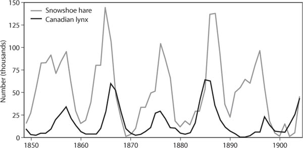
Figure 1. FLuctuations in Lynx and snowshoe hare popuLations based on the number of pelts purchased by the Hudson Bay Company between 1845 and 1930 (data from NERC, 1999).
Population cycles occur in a diverse array of animals ranging from arctic mammals to forest insect pests. Traditionally, predation is one factor thought to induce such cycles (Gilg et al., 2003). Historic support for the view that a coupled predator–prey interaction can drive population cycles came from an analysis of about 100 years of fur-trapping records by the Hudson Bay Company in boreal Canada. An analysis of the number of lynx and snowshoe hare pelts showed spectacular cyclicity with peaks and valleys of abundance occurring at roughly 10-year intervals (figure 1). When hares were numerous, lynx increased in numbers, reducing the hare population, which in turn caused a decline in the lynx population. With predation relaxed, the hare population recovered, and the cycle began anew. It should be noted, however, that there is controversy over the singular role of predation in driving population cycles in boreal mammals.
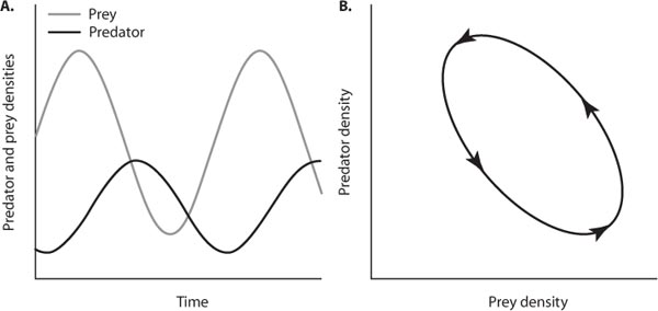
The first ecologists to model the cyclic dynamics of predator–prey interactions were Alfred Lotka (1925) and Vito Volterra (1926), who independently derived the “predator–prey equations” (Lotka-Volterra equations), a pair of differential equations describing the coupled dynamics of a single specialized predator and one prey species. Both ecologists based their models on observations of reciprocal predator–prey cycles in nature. Volterra’s ideas were motivated by watching the rise of fish populations in response to decreased fishing pressure during World War I, whereas Lotka was inspired by observing parasitoid–moth cycles. The Lotka-Volterra equations demonstrate the inherent propensity for predator–prey populations to oscillate, in what is called “neutral stability” (Begon et al., 1996).
For the prey or host population, the rate of population change through time (dH/dt) is represented by the equation:
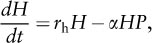
where H is prey density, rh is the rate of increase of the prey population (birthrate), α is a constant that measures the prey’s vulnerability and predator’s searching ability, and P is predator density. Thus, exponential growth of the prey population (rhH) is countered by deaths from predation (αHP). Change in the predator population through time (dP/dt) is shown by:
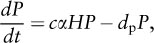
where c is a constant, namely the rate that prey are converted to predator offspring, and dp is the rate of decrease in the predator population (death rate). The death rate of the predator population (–dpP) is offset by the rate at which predators kill prey and convert them to offspring (cαHP). The two equations provide a periodic solution in that predator and prey populations oscillate in reciprocal fashion through time (figure 2A). When the dynamics of predator and prey populations resulting from the Lotka-Volterra equations is plotted in two-phase space (predator density versus prey density), a neutral limit cycle results whereby both predator and prey populations cycle perpetually in time (figure 2B).
Figure 2. (A) Oscillating predator and prey populations and (B) a neutrally stable predator–prey limit cycle generated by the Lotka-Volterra equations.
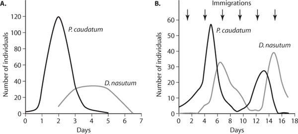
Seeing that simple models could generate predator–prey oscillations prompted numerous researchers to duplicate such persistent cycles under simple laboratory conditions. However, these attempts often failed. A representative example involved the predaceous ciliate protozoan Didinium nasutum and its prey, another ciliate, Paramecium caudatum. Five Paramecium were placed in laboratory cultures, and after 2 days three predators were added. Initially, prey populations exploded in the absence of predators, but with the addition of predators, Paramecium populations were quickly driven to extinction. Moreover, in the absence of prey, predators subsequently perished (figure 3A).
These unexpected results, and those from many other laboratory attempts, raised the question of why predator–prey cycles could not be easily reproduced in the laboratory, why such simple systems were inherently unstable, and why the predator–prey interaction did not persist. Simply stated, more is needed to understand why prey is not driven to extinction at high predator densities and why predators persist when focal prey are rare. As the following sections demonstrate, ecologists have since identified multiple factors missing from the Lotka-Volterra model that introduce realism into predator–prey interactions and lend accuracy in predicting real-world dynamics. As a result, more recent models incorporate biological features such as saturating predator functional responses (inability of predators to capture all available prey when prey are abundant), nonlinear reproductive responses, predator interference, refuges, spatial processes such as immigration, alternative prey, and multiple trophic levels (Canham et al., 2003; Grimm and Railsback, 2005).
Although the Lotka-Volterra equations generate coupled predator–prey oscillations, they are inherently oversimplified. It is unrealistic to expect predators and prey to cycle as predicted (figure 2). For instance, several assumptions of the early predator–prey models are not met by real organisms. The models assume exponential growth of prey in the absence of predation and exponential decline of the predator population in the absence of prey. Prey, however, are often resource limited, and their population growth can be slowed independent of predation. As shown in the discussion of functional responses below, predators are rate limited in their ability to capture and process prey, which constrains their ability to suppress prey populations at high densities. Also, predators often interfere with one another at high predator densities, further relaxing predation pressure on prey. There is also the unrealistic model expectation that predators and prey respond instantaneously to changes in each other’s densities. For microorganisms with high reproductive rates, this expectation is not far fetched. However, for larger predators, their reproductive response to increased prey density is lagged, providing the opportunity for prey to escape predator control, ultimately leading to an unstable dynamic.
There are a multitude of other reasons why simple models inadequately predict predator–prey dynamics and do not capture the complexity of predator–prey interactions in nature. Foremost is that predator–prey interactions do not take place in closed systems in the absence of spatial processes such as emigration and immigration. At low prey densities, predators often disperse to areas of higher prey density, thus relaxing predation on the local prey population rather than driving it to extinction. Moreover, immigration from neighboring patches can rescue declining local populations. Even in very simple lab settings, immigration can encourage the persistence and cycling of predators and prey. Returning to the Didinium–Paramecium system, the addition of a single individual predator and prey every third day of the experiment resulted in a persistent predator–prey cycle (figure 3B).
Figure 3. Interaction between predator (Didinium nasutum) and prey (Paramecium caudatum) in Laboratory microcosms (A) without immigration and (B) with immigration (the addition of a single individual of the predator and prey once every 3 days as indicated by arrows). Low-LeveL immigration of predators and prey into the system promoted the cycLing and persistence of predator and preypopuLations. (From Gause, 1934)
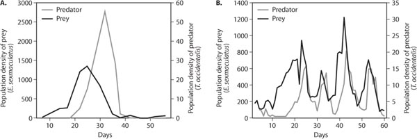
Figure 4. In a simple-structured habitat without refuges (A), predacious mites drive herbivorous mites to low densities, leading to the starvation and ultimate extinction of predatory mites. In a complex-structured habitat (B), herbaceous mites find refuge from predation, and the predator–prey oscillation persists until food (oranges) quality for the prey deteriorates (Huffaker, 1958).
In addition to spatial processes, complex habitat structure and the refuge it provides for prey from predation also lend persistence to predator–prey interactions. A classic example involves interactions between the citrus-feeding mite Eotetranychus sexmaculatus and its predatory mite Typhlodromus occidentalis (Huffaker, 1958). The population dynamics of the mites was compared between two experimental habitats: a simple habitat consisting of a monoculture of oranges arranged on trays and a complex-structured habitat where oranges were interspersed among rubber balls and little posts from which prey could disperse. In the simple universe, predaceous mites easily dispersed throughout the habitat, prey were driven to a threateningly low density, and the predator then became extinct (figure 4A). In the complex habitat, prey dispersed and found refuges from predation, and three complete predator–prey oscillations resulted before the food quality of oranges deteriorated and the system collapsed (figure 4B). This study highlights the importance of refuges in promoting the coexistence of predators and prey, but it also emphasizes that other factors such as food quality bear on the persistence of the interaction.
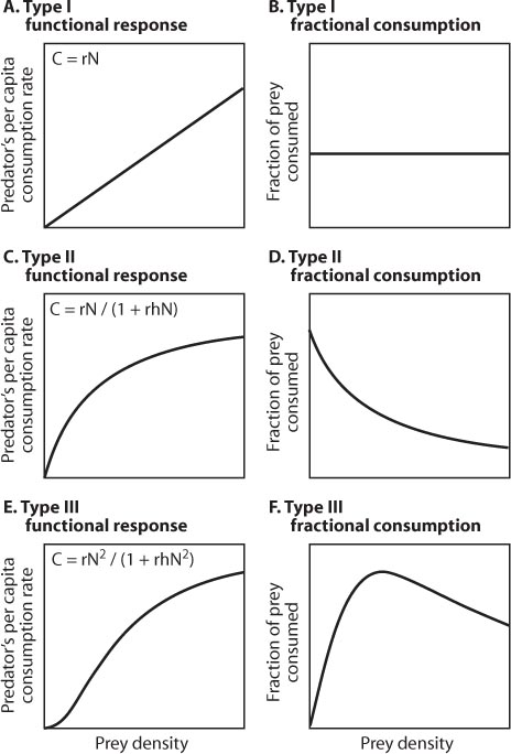
Prey species also escape predation as a result of constraints on the ability of predators to catch and handle prey (functional response) and increase their population size (numerical response) as prey densities rise (Holling, 1959, 1965). In his component analysis of predation, Holling described three types of functional response (figure 5).
Figure 5. Consumption rate of predators when offered prey at increasing densities. Per capita consumption rates are shown for predators exhibiting Type I, II, and III functional responses (A, C, and E, respectively), as is the fractional consumption rate (proportion of prey taken of the total number offered) for each functional response (B, D, and F). Associated equations describe the specific functional response: C = per capita consumption rate, N = prey density, r = “risk of discovery” (a measure of prey vulnerability), and h = handling time.
For predators exhibiting a Type I functional response, the consumption rate of a single individual is limited only by prey density (figure 5A). Thus, over a wide range of densities, per capita consumption and prey density are linearly related. Many filter feeders (e.g., rotifers and sponges) that consume suspended zooplankton exhibit this response. For predators showing a Type I response, the proportion of prey captured of the total number offered remains constant and independent of prey density (figure 5B).
Most invertebrate predators (e.g., hunting spiders, preying mantises, ladybug beetles) exhibit a Type II functional response, in which consumption rate levels off with increasing prey density to an upper plateau (saturating response) set by handling time (the time required to subdue and consume each prey item) and satiation (figure 5C). At high prey densities, most of a predator’s time is spent handling captured prey, and little time is spent searching for additional prey. Notably, for predators with a Type II response, the fraction of prey captured of the available total decreases with increasing prey density (figure 5D). As prey density increases, such predators are less able to reduce prey population growth, thus providing prey with an ever-growing opportunity to escape from predation.
Many vertebrate predators (e.g., birds and mammals) and some invertebrate predators show a sigmoidal or Type III functional response (figure 5E). For such predators, consumption rate responds slowly to increases in prey density when prey is scarce. At somewhat higher prey densities, consumption rate rises rapidly, and at very high prey densities, consumption rate saturates and is limited by handling time as in a Type II response. The rapid rise in consumption rate at intermediate prey densities occurs because predators learn to discover and capture prey with increased efficiency or they simply increase their searching rate as they encounter more prey. In some cases, predators respond to volatile chemicals emitted by their prey and thereafter rapidly increase and direct their searching rate accordingly.
Polyphagous predators often switch to alternative prey when the density of their preferred prey species falls below a certain threshold. Cases of prey switching can transform a Type II response into a Type III because the consumption rate of focal prey is relaxed at low prey densities. Regardless of the mechanism (learning, increased search rate, or prey switching), predators exhibiting a Type III response are thought to stabilize predator–prey interactions. Stability is imposed because the fraction of prey consumed by a predator is low at low densities, preventing predators from driving prey to extinction (figure 5F). Yet, with an increase in prey density, the fraction of prey consumed increases (is density dependent), thus reducing the opportunity for prey to escape predator control. Only at very high densities are predators satiated such that the fraction of prey consumed decreases and the prey population escapes.
So far, we have considered only the consumption rate of an individual predator under conditions of increasing prey density. To gain a complete picture of how predators might control prey populations, we also need to know how many predators are present in the population and how they respond to increasing prey densities. Most predators exhibit a numerical response by becoming more abundant as the density of their preferred prey increases. Two independent mechanisms underlie this pattern. First, predators often aggregate in areas where prey abound, a response that results from a short-term change in the spatial distribution of predators. For instance, the local density of the wolf spider Pardosa littoralis can be dramatically enhanced over a 3-day period when prey is experimentally added to its habitat (Döbel and Denno, 1994). Second, if prey density remains high for an extended period of time, predator populations often build as a consequence of increased reproduction. The density of Arctic foxes, for instance, increases greatly during peak lemming years because of elevated breeding success (Gilg et al., 2003). Thus, predator aggregation and enhanced reproduction can both account for the numerical response of a predator to increased prey density. Like functional responses, numerical responses level off at intermediate prey densities because continued increases in prey densities do not result in a higher predator density because of reproductive limitations or interference among conspecific predators. Nonetheless, strong aggregative responses are often thought to stabilize predator–prey interactions because predation is relaxed in vacated habitats where prey density is low, whereas predation is increased in colonized habitats where prey is more abundant.
Combining a predator’s functional and numerical responses into its total response predicts a predator’s overall response to increased prey density and thus its overall impact on the prey population. A predator’s total response (number of prey consumed/unit area) can be calculated by multiplying its functional response (number of prey consumed/predator) by its numerical response (number of predators/unit area). Because both functional and numerical responses level off at intermediate prey densities, further increases in prey density result in an increasingly smaller proportion of the prey population that is killed by predators. Thus, the opportunity for escape exists at high prey densities, and one defensive strategy is for prey to satiate the predator population by emerging synchronously at very high densities. Periodical cicadas (Magicicada) appear to employ this strategy in that the proportion of mortality attributable to predation is drastically reduced during times of peak emergence when cicadas reach incredibly high densities.
Other life history traits of prey, such as dispersal capability, stage class, and body size may also provide escape from predation and thus contribute to the persistence of predator–prey interactions. Regarding dispersal, a highly mobile lifestyle appears to promote escape from predator control. Planthopper species, for example, vary tremendously in their dispersal ability with both highly mobile and extremely sedentary species represented. In a survey of species, invertebrate predators inflicted significantly more mortality on immobile species than on their migratory counterparts (Denno and Peterson, 2000). Invulnerable stage classes also provide a refuge from predation. The true bug Tytthus attacks only the eggs of planthoppers; thus, once planthopper eggs have hatched, emerging nymphs are immune to predation from this specialist predator. Also, because the act of predation requires overpowering victims, predators usually profit by attacking smaller or weaker individuals in the prey population. Size-selective predation has been observed across a wide range of vertebrate (snakes, fish, birds, and mammals) and invertebrate predators (insects, spiders, starfish). Importantly, because predators often focus their attacks on smaller prey, larger prey obtain a partial refuge from predation.
So far, our focus has been on interactions between a single predator and prey species and how inherent limitations imposed by a predator’s functional and numerical responses and size-selective predation can offer prey a partial escape from predation. However, predators and prey are nested into food webs and do not occur in isolation from other players. In fact, refuges for prey exist because of other species in the system. We have already seen how the presence of alternative prey species can relax predation on focal prey when its density drops to low levels. Moreover, mesopredators are also subject to predation themselves from top carnivores. Thus, interactions among predators can result in intraguild predation, which often relaxes predation on shared prey. A good example involves heteropterans bugs (Zelus and Nabis) and lacewing larvae (Chrysoperla), all of which prey on cotton aphids (Rosenheim et al., 1993). In the absence of heteropterans predators, lacewing predation drives the aphid population to a low level. When heteropterans are added to the system, they focus their attack on the more vulnerable lacewings, aphids experience a partial refuge from predation, and aphid populations rebound. Thus, the presence of multiple predator and prey species in the community can alter the interaction between a specific predator–prey pair and often lends stability to any specific interaction.
By now it should be clear that many factors influence the dynamics of a specific predator–prey interaction. Even in the simplest of systems, it is difficult to draw solely on the focal pair of players to explain each other’s population fluctuations. For instance, the 4-year population cycles of lemmings in Greenland are driven by a 1-year delay in the numerical response of stoat and stabilized by density-dependent predation imposed by arctic foxes, snowy owls, and skuas (Gilg et al., 2003). Moreover, recent assessments of snowshoe hare population dynamics (figure 1), including a large-scale predator exclusion and food enhancement experiment, suggest that hare population cycles result from interactions among three trophic levels (Krebs et al., 1995, 2001). When lynx and other predators were experimentally excluded, hare populations doubled. Hare populations tripled when plant biomass was increased via fertilization. Strikingly, hare populations increased 11-fold when predators were excluded and plant resources were enhanced. This finding highlights the view that predators and prey can indeed affect each other’s abundance, but the dynamic of the interaction is complex and can not be studied in isolation from other factors.
Visiting an invertebrate system further underscores why understanding predator–prey interactions requires a multitrophic approach (Finke and Denno, 2004, 2006). Spartina cordgrass is the only host plant for Prokelisia planthoppers, which in turn are consumed by the mesopredator Tytthus and the intraguild predator Pardosa. In this intertidal system, there is considerable variation in leaf litter as a result of elevational differences in tidal flushing and decomposition. In litter-rich habitats, Pardosa spiders abound and readily aggregate in areas of elevated planthopper density. In these structurally complex habitats, Tytthus finds refuge from Pardosa predation, the predator complex effectively suppresses planthoppers, and cordgrass flourishes. By contrast, in litter-poor habitats, spiders are less abundant, Tytthus experiences intraguild predation, and overall predation on planthoppers is relaxed, leading to planthopper outbreak and reduced plant biomass. Thus, both vegetation structure and the predator assemblage interact in complex ways to influence the strength of the spider–planthopper interaction and the probability for a trophic cascade, namely the extent to which predator effects cascade to affect herbivore suppression and plant biomass. This example and many others further emphasize that alternative population equilibria exist for prey and that release from predation is dependent on spatial refuges and the composition of other players in the system.
Although there is evidence that cycling does occur in some simple predator–prey systems in the boreal north, coupled cycling is not often characteristic of predator–prey dynamics in more complex food webs. Here, plant-mediated effects, alternative prey, intraguild predation, and refuges collectively dampen predator–prey cycles. Moreover, such multitrophic interactions are the rule and are thought to lend stability to food webs, making them more resistant to environmental disturbance and invasion by other species (Fagan, 1997).
Predators can act as keystone species influencing the species composition and biodiversity of the prey community. A classic case involves starfish, which graze mussels and barnacles in intertidal habitats, precluding them from dominating the community, allowing other invertebrate species to persist, and enhancing the overall diversity of the benthic community (Paine, 1974). From a conservation perspective, however, exotic predators that invade natural habitats can have very negative effects on resident prey species, effects that can cascade throughout the food web. When the brown treesnake was accidentally introduced to Guam, its population erupted in the absence of native predators, ultimately leading to the widespread extirpation of many native vertebrate species including birds, mammals, and lizards. Similarly, rainbow trout have been purposefully introduced throughout the world, often with devastating effects on native stream communities. In parts of New Zealand, trout incursion resulted in a trophic cascade, whereby this efficient predator reduced populations of native invertebrates that graze on benthic algae, which in turn promoted dramatic increases in algal biomass.
Another alarming consequence of our rapidly changing world is the loss of biodiversity as a result of habitat disturbance, fragmentation, and loss. In particular, consumers at higher trophic levels such as predators are at risk of extinction. In coastal California, for example, urbanization and habitat fragmentation have promoted the disappearance of coyote, the historic top carnivore in this sage–scrub habitat (Crooks and Soulé, 1999). Its disappearance has fostered increased numbers of smaller mesopredators (e.g., foxes and skunks), which in turn are contributing to the extinction of scrub-breeding birds.
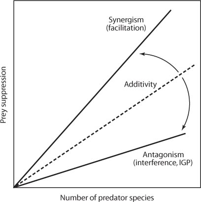
A practical extension of the consequences of multiple-predator interactions is whether single or multiple predators are more effective in suppressing agricultural pests. The effect of increased predator diversity on biological control, and ecosystem function at large, depends on how predator species interact and complement each other (figure 6). We have already seen how increasing predator diversity by adding an intraguild predator to the enemy complex can relax predation on shared herbivore prey. However, not all predator–predator interactions are antagonistic. In stream systems, predators interact synergistically, whereby stonefly predators drive mayflies from under stones making them more susceptible to fish attack (Soluk and Collins, 1988). Thus, predators that interact synergistically can enhance prey suppression beyond additive expectations. Likewise, if predators complement each other by attacking prey at different developmental stages or during different times of the year, increasing predator diversity can enhance prey suppression. The key to elucidating the relationship between predator diversity and ecosystem function or manipulating the composition of the predator assemblage for more effective biological control rests on the nature of predator–predator interactions in the system. The issue remains open in biological control because there is system-specific evidence that increasing predator diversity can either increase or decrease pest suppression.
Figure 6. Relationships between the number of predator species in the system and prey suppression. Synergism results from facilitation, additivity arises from predator complementarity, and antagonism occurs from intraguild predation (IGP) or interference.
There is little doubt that predators have exerted selection on prey that has resulted in evolutionary change. For instance, prey species have evolved a wide range of defenses in response to selection from predation. Such defenses can be categorized as primary, secondary, or tertiary depending on when in the predation sequence (detection, capture, or handling) they operate. Primary defenses (e.g., crypsis and reduced activity when predators forage) operate before prey is detected by a predator. Secondary defenses operate to deter capture after prey is detected by the predator. Examples include escape mechanisms (aphids dropping from leaves in the presence of a foraging ladybug), startle behaviors (moths displaying wings with eye spots to frighten away birds), and evasive behaviors (moths detecting the sonar of bats and initiating strategic flight-avoidance tactics). Tertiary defenses interrupt predation after capture and during the handling phase. Such defenses include mechanisms that deter, repel, or even kill the predator directly (contact toxins, venoms, or morphological structures such as spines). The consequences of some tertiary defenses for predators can be severe. The neurotoxin injected by the death-stalker scorpion (Leiurus quinquestriatus) can cause rapid paralysis and death to an attacking small mammal.
Clearly, predation has promoted a wide array of prey defenses, and the question arises as to whether there have been counteradaptations in predators. Have predators and prey engaged in an “evolutionary arms race” such that reciprocal selection has promoted a continuing escalation of predator offense and prey defense? Some evidence is consistent with this hypothesis. For instance, the drilling abilities of predaceous gastropods and the shell thickness of their bivalve prey have increased through geologic time (Vermeij, 1994). Similarly, marine snails have become more heavily armored, while the correlated response in predaceous crabs has been the evolution of larger claws for crushing the better-defended snails. In both of these instances, predators may have evolved greater weaponry in reciprocal response to improved prey defense (coevolution hypothesis), or predator armaments may have evolved in response to other predators or competitors (escalation scenario).
Overall, however, evidence suggests that reciprocal selection on predators may be weaker than that on prey, thus precluding a classic evolutionary arms race (Brodie and Brodie, 1999). In part, the asymmetry arises because many predators are generalist feeders, and selection imposed by any one of its prey options is likely small. In general, coevolution between exploiter and exploited is unlikely when the intimacy of the interaction is low. Moreover, selection on predators from effective primary and secondary prey defenses is probably weak. For instance, if a predator fails to detect cryptic prey or catch a stealthy individual, it simply searches for another, without penalty. The exception occurs when predators interact with dangerous prey, prey that possess tertiary defenses such as toxins that can kill the attacker. In such cases, predators experience strong selection from prey and are expected to evolve either innate avoidance behavior or traits that allow them to exploit dangerous prey. Such a case of coevolution has likely occurred between the toxic newt Taricha granulosa and its garter snake predator Thamnophis sirtalis. The skin of the newt contains one of the most potent neurotoxins known, one that kills all other predators outright. Across populations, geographic variation in the level of newt toxin covaries with levels of resistance in the snake. Thus, garter snakes are evolving in response to newt defenses, and the “arms race” is apparently taking place (Brodie and Brodie, 1999).
Predation is a central process in community ecology because it is responsible for energy flow among multiple trophic levels. Moreover, the many reticulate linkages resulting from predation across multiple trophic levels (omnivory) are an important stabilizing force in food-web dynamics. Predators, however, by virtue of their precarious position at the apex of the food chain, are often at greater risk of extinction when natural systems are disturbed, often with dire consequences for the diversity and functioning of the community at large. Also, predators are important members of natural-enemy complexes that can provide effective pest control in agroecosystems. From the perspective of the consequences of predation, however, it is crucial to realize that the objectives of conservation biology and biological control seek very different ends. Conservation biologists seek to retain trophic diversity, preserve trophic linkages (e.g., intraguild predation) that stabilize food-web interactions, and reduce the probability that predator effects will cascade to affect plant productivity. Reconstructing stable food-web dynamics and ecosystem function are particularly important in habitat restoration projects. By contrast, biological control aims to induce trophic cascades, whereby antagonistic interactions among predators are minimized, pests are collectively suppressed by the enemy complex, and crop yield is enhanced. This contrast in objectives provides an ideal impetus for exploring the complex role of predation in community dynamics from both applied and theoretical perspectives.
Begon, M., J. A. Harper, and C. R. Townsend. 1996. Ecology, 3rd ed. London: Blackwell Science.
Brodie, E. D. III, and E. D. Brodie, Jr. 1999. Predator–prey arms races. BioScience 49: 557–568.
Caltagirone, L. E., and R. L. Doutt. 1989. The history of the vedalia beetle importation to California and its impact on the development of biological control. Annual Review of Entomology 34: 1–16.
Canham, Charles D., Jonathan J. Cole, and William K. Lauenroth. 2003. Models in Ecosystem Science. Princeton, NJ: Princeton University Press.
Cronin, J. T., K. J. Haynes, and F. Dillemuth. 2004. Spider effects on planthopper mortality, dispersal and spatial population dynamics. Ecology 85: 2134–2143.
Crooks, K. R., and M. E. Soulé. 1999. Mesopredator release and avian extinctions in a fragmented habitat. Nature 400: 563–566.
Denno, R. F., and M. A. Peterson. 2000. Caught between the devil and the deep blue sea, mobile planthoppers elude natural enemies and deteriorating host plants. American Entomologist 46: 95–109.
Döbel, H. G., and R. F. Denno. 1994. Predator–planthopper interactions. In Planthoppers: Their Ecology and Management. R. F. Denno and T. J. Perfect, eds. New York: Chapman & Hall, 325–399.
Fagan, W. F. 1997. Omnivory as a stabilizing feature of natural communities. American Naturalist 150: 554–567.
Finke, D. L., and R. F. Denno. 2004. Predator diversity dampens trophic cascades. Nature 429: 407–410.
Finke, D. L., and R. F. Denno. 2006. Spatial refuge from intraguild predation: Implications for prey suppression and trophic cascades. Oecologia 149: 265–275.
Gause, G. F. 1934. The Struggle for Existence. Baltimore: Williams & Wilkins. Reprinted 1964, New York: Hafner.
Gilg, O., I. Hanski, and B. Sittler. 2003. Cyclic dynamics in a simple vertebrate predator–prey community. Science 302: 866–868.
Grimm, V., and S. F. Railsback. 2005. Individual-based Modeling and Ecology. Princeton, NJ: Princeton University Press.
Holling, C. S. 1959. The components of predation as revealed by a study of small mammal predation of the European pine sawfly. Canadian Entomologist 91: 293–320.
Holling, C. S. 1965. The functional response of predators to prey density and its role in mimicry and population regulation. Memoirs of the Entomological Society of Canada 45: 5–60.
Huffaker, C. B. 1958. Experimental studies on predation: Dispersion factors and predator–prey oscillations. Hilgardia 27: 343–383.
Krebs, C. J., R. Boonstra, S. Boutin, and A.R.E. Sinclair. 2001. What drives the 10-yr cycle of snowshoe hares? BioScience 51: 25–36.
Krebs, C. J., S. Boutin, R. Boonstra, A.R.E. Sinclair, J.N.M. Smith, M.R.T. Dale, K. Martin, and R. Tarkington. 1995. Impact of food and predation on the snowshoe hare cycle. Science 269: 1112–1115.
NERC Centre for Population Biology, Imperial College. 1999. The Global Population Dynamics Database. http://www.sw.ic.ac.uk/cpb/cpb/gpdd.html.
Paine, R. T. 1974. Intertidal community structure: Experimental studies of the relationship between a dominant competitor and its principal predator. Oecologia 15: 93–120.
Rosenheim, J. A., L. R. Wilhoit, and C. A. Armer. 1993. Influence of intraguild predation among generalist insect predators on the suppression of an herbivore population. Oecologia 96: 439–449.
Schmitz, O. J., A. P. Beckerman, and K. M. O’Brien. 1997. Behaviorally mediated trophic cascades: Effects of predation risk on food web interactions. Ecology 78: 1388–1399.
Soluk, D. A., and N. C. Collins. 1988. Balancing risks? Responses and nonresponses of mayfly larvae to fish and stonefly predators. Oecologia 77: 370–374.
Symondson, W.O.C., K. D. Sunderland, and M. H. Greenstone. 2002. Can generalist predators be effective biocontrol agents? Annual Review of Entomology 47: 561–594.
Vermeij, G. J. 1994. The evolutionary interaction among species: Selection, escalation, and coevolution. Annual Review of Ecology and Systematics 25: 219–236.