3. Shallow lakes as an example
4. Mechanisms for alternative stable states in ecosystems
5. How to know if a system has alternative stable states
6. Using alternative stable states in management
Complex systems ranging from cells to ecosystems and the climate can have tipping points, where the slightest disturbance can cause the system to enter a phase of selfpropagating change until it comes to rest in a contrasting alternative stable state. The theory explaining such catastrophic change at critical thresholds is well established. In particular, an early influential book by the French mathematician René Thom catalyzed the interest in what he called “catastrophe theory.” Although many claims about the applicability to particular situations were not substantiated later, catastrophe theory created an intense search for real-life examples, much like chaos theory later. In the 1970s, C. S. Holling was among the first to argue that the theory could explain important aspects of the dynamics of ecosystems, and an influential review by Sir Robert May in Nature promoted further interest among ecologists. Nonetheless, not until recently have strong cases for this phenomenon in ecosystems been built.
alternative stable states. A system is said to have alternative stable states if under the same external conditions (e.g., nutrient loading, harvest pressure, or temperature) it can settle to different stable states. Although genuine “stable states” occur only in models, the term is also used more liberally to refer to alternative dynamic regimes.
attractor. A state or dynamic regime to which a model asymptotically converges, given sufficient simulation time. Examples are a stable point, a cycle, or a strange attractor.
catastrophic shift. A shift to an alternative attractor that can be invoked by an infinitesimal small change at a critical point known as catastrophic bifurcation.
hysteresis. The phenomenon that the forward shift and the backward shift between alternative attractors happen at different values of an external control variable.
regime shift. A relatively fast transition from one persistent dynamic regime to another. Regime shifts do not necessarily represent shifts between alternative attractors.
resilience. The capacity of a system to recover to essentially the same state after a disturbance.
The idea of catastrophic change at critical thresholds is intuitively straightforward in physical examples. Suppose you are in a canoe and gradually lean over to one side more and more. It is difficult to see the tipping point coming, but eventually leaning over too much will cause you to suddenly capsize and end up in an alternative stable state from which it is not easy to return. Still, people have been hesitant to believe that large complex systems such as ecosystems or the climate would sometimes behave in a similar way. Indeed, fluctuations around gradual trends rather than “tipping over” seem the rule in nature. Nonetheless, occasionally sudden changes from one contrasting fluctuating regime to another one are observed. Such abrupt changes have been termed regime shifts.
As we shall see in this chapter, regime shifts are indicative of the existence of tipping points and alternative stable states but by no means a proof. Indeed, rigorous experimental proofs are possible only in small controlled systems. Such a difficulty of proving that a mechanism is at work in nature is common in ecology. For instance, it has proven remarkably hard to demonstrate unequivocally the role of a mechanism as basic as competition. Nonetheless, the role of alternative stable states in driving some ecosystems dynamics has become an important focus of research. I first briefly show the key aspects of the theory and elaborate the case of shallow lakes as an example. Subsequently, I briefly highlight some other mechanisms and discuss how one may find out if a system has alternative stable states. Finally, I reflect on how insights in such stability properties can be used in managing ecosystems.
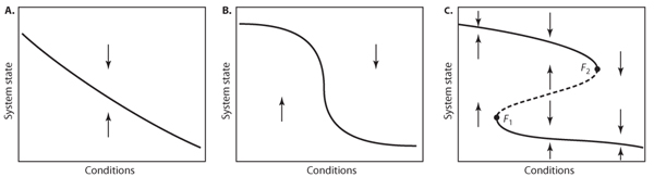
In most cases, the equilibrium of a dynamic system moves smoothly in response to changes in the environment (figure 1A). Also, the system is often rather insensitive over certain ranges of the external conditions, although it responds relatively strongly around some threshold conditions (figure 1B). For instance, mortality of a species usually drops sharply around a critical concentration of a toxicant. In such a situation, a strong response happens when a threshold is passed. Such thresholds are obviously important to understand. However, a very different, much more extreme kind of threshold than this occurs if the system has alternative stable states. In that case, the curve that describes the response of the equilibrium to environmental conditions is typically “folded” backward (figure 1C). Such a catastrophe fold implies that, for a certain range of environmental conditions, the system has two alternative stable states separated by an unstable equilibrium (dashed lines), which marks the border between the basins of attraction of the alternative stable states.
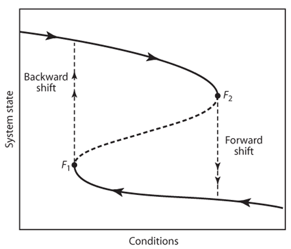
This situation is the root of catastrophic shifts or, with less negative connotation, critical transitions (figure 2). When the system is in a state on the upper branch of the folded curve, it can not pass to the lower branch smoothly. Instead, when conditions change sufficiently to pass the threshold (F2), a “catastrophic” transition to the lower branch occurs. Clearly this point is a very special point. In the exotic jargon of dynamic systems theory it is called a bifurcation point. The point we have in our picture marks a so-called catastrophic bifurcation. Such bifurcations are characterized by the fact that an infinitesimally small change in a control parameter (reflecting, for instance, the temperature) can invoke a large change in the state of the system if it crosses the bifurcation. The bifurcation points in a catastrophe fold (F1 and F2) are known as fold bifurcations. (They are also called “saddle-node” bifurcations because in these points a stable “node” equilibrium meets an unstable “saddle” equilibrium.)
Figure 1. Schematic representation of possible ways in which the equilibrium state of a system can vary with conditions such as nutrient loading, exploitation, or temperature rise. In panels A and B only one equilibrium exists for each condition. However, if the equilibrium curve is folded backward (panel C), three equilibria can exist for a given condition. The arrows in the graphs indicate the direction in which the system moves if it is not in equilibrium (i.e., not on the curve). It can be seen from these arrows that all curves represent stable equilibria except for the dashed middle section in panel C. If the system is pushed away a little bit from this part of the curve, it will move further away instead of returning. Hence, equilibria on this part of the curve are unstable and represent the border between the basins of attraction of the two alternative stable states on the upper and lower branches.
Figure 2. If a system has alternative stable states, critical transitions and hysteresis may occur. If the system is on the upper branch but close to the bifurcation point F2, a slight incremental change in conditions may bring it beyond the bifurcation and induce a critical transition (or catastrophic shift) to the lower alternative stable state (“forward shift”). If one tries to restore the state on the upper branch by means of reversing the conditions, the system shows hysteresis. A backward shift occurs only if conditions are reversed far enough to reach the other bifurcation point F1.
The fact that a tiny change in conditions can cause a major shift is not the only aspect that sets systems with alternative stable states apart. Another important feature is the fact that in order to induce a switch back to the upper branch, it is not sufficient to restore the environmental conditions that existed before the collapse (F2). Instead, one needs to go back further, beyond the other switch point (F1), where the system recovers by shifting back to the upper branch. This pattern in which the forward and backward switches occur at different critical conditions (figure 2) is known as hysteresis. From a practical point of view, hysteresis is important because it implies that this kind of catastrophic transition is not so easy to reverse.
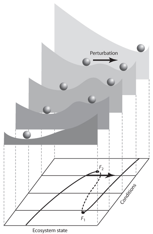
The idea of catastrophic transitions and hysteresis can be nicely illustrated by stability landscapes. To see how stability is affected by change in conditions, we make stability landscapes for different values of the conditioning factor (figure 3). For conditions in which there is only one stable state, the landscape has only one valley. However, for the range of conditions where two alternative stable states exist, the situation becomes more interesting. The stable states occur as valleys, separated by a hilltop. This hilltop is also an equilibrium (the slope of the landscape is zero). However, this equilibrium is unstable. It is a repellor. Even the slightest movement away from it will lead to a self-propagating runaway change moving the system toward a stable equilibrium. Such a stable equilibrium is an attractor.
To see the catastrophic transitions and hysteresis in this representation, imagine what happens if you start in the situation of the landscape up front. The system will then be in the only existing equilibrium. There is no other attractor, and therefore, this state is said to be globally stable. Now, suppose that conditions change gradually, so that the stability landscape changes to the second or third one in the row. Now, there is an alternative attractor, implying that the state in which we were has become locally (rather than globally) stable. However, as long as no major perturbation occurs, the system will not move to this alternative attractor. In fact, if we would monitor the state of the system, we would not see much change at all. Nothing would reveal the fundamental changes in the stability landscape. If conditions change even more, the basin of attraction around the equilibrium in which the system rests becomes very small (fourth stability landscape) and eventually disappears (last landscape), implying an inevitable catastrophic transition to the alternative state. Now, if conditions are restored to previous levels, the system will not automatically shift back. Instead, it shows hysteresis. If no large perturbations occur, it will remain in the new state until the conditions are reversed beyond those of the second landscape.
Figure 3. External conditions affect resilience of multistable systems to perturbation. The bottom plane shows the equilibrium curve as in figure 2. The stability landscapes depict the equilibria and their basins of attraction at five different conditions. Stable equilibria correspond to valleys; the unstable middle section of the folded equilibrium curve corresponds to hilltops. If the size of the attraction basin is small, resilience is small, and even a moderate perturbation may bring the system into the alternative basin of attraction.
In reality, conditions are never constant. Stochastic events such as weather extremes, fires, or pest outbreaks can cause fluctuations in the conditioning factors but may also affect the state directly, for instance by wiping out parts of populations. If there is only one basin of attraction, the system will settle back to essentially the same state after such events. However, if there are alternative stable states, a sufficiently severe perturbation may bring the system into the basin of attraction of another state. Obviously, the likelihood of this happening depends not only on the perturbation but also on the size of the attraction basin. In terms of stability landscapes (figure 3), if the valley is small, a small perturbation may be enough to displace the ball far enough to push it over the hilltop, resulting in a shift to the alternative stable state. Following Holling, I use the term resilience to refer to the size of the valley or basin of attraction around a state that corresponds to the maximum perturbation that can be taken without causing a shift to an alternative stable state. Note that gradually changing conditions may have little effect on the state of the system but nevertheless reduce the size of the attraction basin. This loss of resilience makes the system more fragile in the sense that it can be easily tipped into a contrasting state by stochastic events.
A tricky and often overlooked problem is that we cannot generalize stability properties of a system. For instance, we cannot make statements such as: the critical nutrient level for a lake to collapse into a turbid state is 0.1 mg/L phosphorus. In fact, we cannot even say that “lakes have alternative stable states.” In technical terms, the problem is that the positions of critical bifurcation points (e.g., F1 and F2) always depend on various parameters of a model. In practice, this means that the corresponding thresholds are not fixed values. For instance, the critical nutrient level for a shallow lake to flip from a clear to a turbid state depends on its size. In a wider sense, it means that safe limits to prevent critical transitions will usually not have universal fixed values.
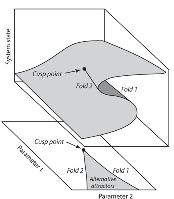
A corollary is that the degree of hysteresis may vary strongly. For instance, shallow lakes can have a pronounced hysteresis in response to nutrient loading (figure 1C), whereas deeper lakes may react smoothly (figure 1B). Often a parameter can be found that can be changed such that the bifurcation points move closer together and eventually merge and disappear. This “bifurcation of bifurcations” is known as cusp bifurcation, after the hornlike shape produced by the fold bifurcations moving together (figure 4). It marks the change from a situation in which the system can respond in a catastrophic way to a situation in which the response to a control parameter (parameter 2 in figure 4) is always smooth, as there are no alternative attractors. Thus, the panels with distinct possible responses to external conditions (figure 1) do in fact represent snapshots of a continuum of possible behavior that may be displayed by a single system. A positive feedback is usually responsible for causing a threshold response. A moderate feedback may turn a smooth response (figure 1A) into a threshold response (figure 1B), and a stronger feedback may cause the response curve to turn into a catastrophe fold (figure 1C).
Another point to note is that there is in principle no limit to the number of alternative attractors in a system. In general, complex systems may have complex stability landscapes, with numerous smaller or larger attraction basins. In analogy to the scenarios for two alternative stable states, gradually changing conditions (e.g., temperatures) may alter the landscapes, making some attraction basins larger and causing others to disappear. Meanwhile, disturbances occasionally flip the system out of an attraction basin that has become small, allowing it to settle into a more resilient state. Obviously, this is still a very stylized world view, but before elaborating it, I will give an example of an ecosystem with alternative stable states.
It is obvious that the elegant and simple models described in dynamic systems theory can capture only some aspects of what happens in complex reality. For instance, the idea of “stable states” is a gross simplification of the dynamic regimes observed in nature. There are always fluctuations, driven by a combination of stochastic forcing and seasonal cycles in the weather, mixed in many systems with intrinsically generated chaotic dynamics or cycles. Therefore, it is perhaps more appropriate to speak about alternative dynamic regimes rather than alternative stable states if we are thinking about real systems. Nonetheless, I shall stick to the simple “stable states” terminology in this chapter. On very long time scales, there is obviously no stability either, as eventually lakes become land, and the Earth system evolves inevitably. Another complication is the heterogeneity of nature, as compared to the simple models used by theoreticians. The models usually assume homogeneous environments with only a few key players. In practice, heterogeneity of environmental conditions may complicate the picture, and so may the great variety of species that are usually involved in ecosystem dynamics. Some places may be better for growth than others, and some species may replace others depending on conditions. Spatial exchange may then help to smooth patterns at larger scales. I cannot elaborate on all those aspects here, but the bottom line is that although fluctuations, heterogeneity, and spatial processes may smooth things, there are also situations where the mechanism leading to alternative stable states is strong enough to dominate the dynamics, and real systems show a behavior that can be quite well explained by the simple theory presented above.
Figure 4. The cusp point where two fold bifurcation lines meet tangentially and disappear marks the change from a system with catastrophic state shifts in response to change in parameter 2 to one that responds smoothly to that parameter.
A particularly well-studied example of bistability of an entire ecosystem is the development of submerged vegetation in turbid shallow lakes. Submerged plants can enhance water clarity by a suite of mechanisms such as control of excessive phytoplankton development and prevention of wave resuspension of sediments. However, the submerged plants also need low turbidity in order to get sufficient light. As a consequence, there is a positive feedback: plants promote water clarity and vice versa. It seems intuitively straightforward that such a positive feedback may lead to alternative stable states: one vegetated and another one without plants. However, things are more complex than that. First, as argued, alternative equilibria arise only if the feedback effect is strong enough. Second, stability of one of the states can be lost if external factors such as climate or nutrient input change (cf. figure 3).
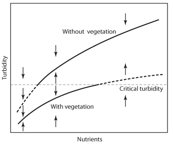
To see how such loss of stability can happen, consider a simple graphic model of the response of shallow lakes to nutrient loading (figure 5). An overload with nutrients such as phosphorus and nitrogen derived from waste water or fertilizer use tends to make lakes turbid. This is because the nutrients stimulate growth of microscopic phytoplankton, which makes the water greenish and turbid. Although this eutrophication process can be gradual, shallow lakes tend to jump abruptly from the clear to the turbid state. This behavior can be explained from a simple graphic model based on only three assumptions: (1) Turbidity increases with the nutrient level because of increased phytoplankton growth. (2) Vegetation reduces turbidity. (3) Vegetation disappears when a critical turbidity is exceeded.
In view of the first two assumptions, equilibrium turbidity can be drawn as two different functions of the nutrient level: one for a macrophyte-dominated and one for an unvegetated situation. Above a critical turbidity, macrophytes will be absent, in which case the upper equilibrium line is the relevant one; below this turbidity the lower equilibrium curve applies. The emerging picture shows that, over a range of intermediate nutrient levels, two alternative equilibria exist: one with macrophytes and a more turbid one without vegetation. At lower nutrient levels, only the macrophyte-dominated equilibrium exists, whereas at the highest nutrient levels, there is only a vegetationless equilibrium.
Figure 5. Alternative equilibrium turbidities caused by disappearance of submerged vegetation when a critical turbidity is exceeded (see text for explanation). The arrows indicate the direction of change when the system is not in one of the two alternative stable states. (From Scheffer, M., S. H. Hosper, M. L. Meijer, B. Moss, and E. Jeppesen. 1993. Alternative equilibria in shallow lakes. Trends in Ecology and Evolution 8: 275–279)
The zigzag line formed by the stable and unstable equilibria in this graphic model corresponds to the folded line in figure 1C and the panel below the stability landscapes (figure 3). However, this simple example may serve to convey a better feeling for the way in which a facilitation mechanism may cause the system to respond to environmental change showing hysteresis and catastrophic transitions. Gradual enrichment starting from low nutrient levels will cause the lake to proceed along the lower equilibrium curve until the critical turbidity is reached at which macrophytes disappear. Now, a jump to a more turbid equilibrium at the upper part of the curve occurs. In order to restore the macrophyte-dominated state by means of nutrient management, the nutrient level must be lowered to a value where phytoplankton growth is limited enough by nutrients alone to reach the critical turbidity for macrophytes again. At the extremes of the range of nutrient levels over which alternative stable states exist, either of the equilibrium lines approaches the critical turbidity that represents the breakpoint of the system. This corresponds to a decrease of resilience. Near the edges, a small perturbation is enough to bring the system over the critical line and to cause a switch to the other equilibrium.
Small lakes have the advantage that they can be experimentally manipulated relatively well. Wholelake experiments in which the fish stock is strongly reduced for a brief period can induce a shift from the turbid to the clear state. The short-term effect of fish removal on turbidity is explained by a trophic cascade (fewer fish results in more zooplankton and therefore less phytoplankton) and the role of bottom-dwelling fish in recycling of nutrients and resuspending sediments. However, fish quickly reproduce, allowing the populations to recover from the brief fishing campaign. The fact that the result of such “shock therapy” can be long term as well is explained by the positive feedback between water clarity and submerged vegetation. The whole-lake experiments and other lines of evidence have made the shallow lake case one of the bestdocumented examples of alternative stable states in ecosystems.
By use of models, it can be shown that alternative stable states may plausibly arise from a range of mechanisms. The shallow lakes case in its simplest representation is an example of facilitation. The submerged plants facilitate their own growth by “engineering” the environmental conditions, making the water clearer. A similar thing may happen in semiarid environments where plants may enhance the water conditions in their environment. This can happen on a very local scale. For instance, an adult plant canopy can ameliorate hot and dry conditions, thereby facilitating growth of smaller plants. However, vegetation may also lead to more cloudy and rainy conditions on a regional scale in some places. For instance, in Northwest Africa, the monsoon circulation that brings rains from the ocean to the land is promoted by vegetation cover, implying a positive feedback. Such positive feedback between plants and water conditions can create alternative stable states on local as well as regional states.
Another mechanism that is well known to create alternative stable states in some situations is competition between two species or functional groups. In classical competition models, the necessary and sufficient condition is that intraspecific competition is weaker than interspecific competition. Thus, both species should do better if they are in a monoculture than when they are together with the other species. If the two competing species or functional groups are dominant in the ecosystem, such a competitive play may dominate the entire ecosystem dynamics. An example is the shift from a diverse phytoplankton community to dominance by particular groups of cyanobacteria in lakes. The cyanobacteria are more shade tolerant but also create more shade given the same amount of nutrients. They thus create conditions in which they are also better competitors. This can lead to a runaway shift toward cyanobacterial dominance under some conditions.
A third mechanism for alternative stable states that should be mentioned is overexploitation. Classical work by Noy-Meir in the 1970s has shown elegantly how, under some conditions, a population can come into free fall if it is exploited beyond a certain critical level. The mechanism is that at low population numbers the overall production declines with population density. Therefore, if exploitation levels do not decline proportionally or more, there will be a self-propagating further decline in the population.
Numerous, more complicated mechanisms for alternative stable states in ecology exist. For instance, metapopulations in scattered habitats may collapse beyond a certain critical level of habitat fragmentation. Also, alternative stable states may occur if a predator controls the natural enemies of its offspring. For instance, it has been hypothesized that Nile perch could come to dominate the Lake Victoria fish community only after the cichlids that can be important egg predators were driven to low enough densities by overfishing and eutrophication. Now the abundant Nile perch helps in keeping the cichlid populations low through predation.
Jumps in Time Series or Regime Shifts
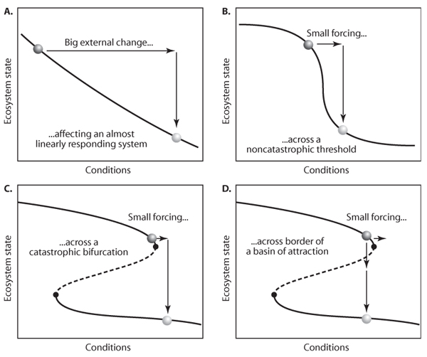
Sudden changes in a system are always an interesting feature, and not surprisingly, various statistical techniques have been developed to check whether a shift in a time series can be explained by chance. However, it is important to keep in mind that even if a critical transition in a time series is significant, this does not necessarily imply that it was a jump between alternative attractors. Probably the most common cause of a sudden change is a sudden change in the conditions. For instance, the closure of a dam for a major reservoir may cause a drastic shift in the downstream river ecosystem. Another possible explanation of a sudden shift is that conditions changed gradually but exceeded a limit at which the system changes drastically although not catastrophically (i.e., not a stability shift related to a catastrophic bifurcation). For example, the onset and termination of a period of ice-cover in a lake can be quite sudden, even if temperature changes develop gradually. Thus, sudden shifts in a time series of some indicator of the state of a system may often simply be caused by a sudden drastic change in an important control parameter (figure 6A) or a control parameter reaching a range where the system responds strongly, even though there is no bifurcation (figure 6B). On the other hand, they can be true critical transitions caused by a tiny but critical change in conditions (figure 6C) and/or a disturbance pushing the system across the border of a basin of attraction (figure 6D). I should stress again, that although real stability shifts (lower two panels) are a distinctly different occurrence (e.g., they can be triggered by infinitely small change and have some irreversibility), there is in fact a continuum of possibilities in the range from linear to catastrophic system responses (figure 4).
It may seem impossible to detect from a time series whether the system went through a real stability shift or, rather, jumped to one of the mechanisms illustrated in the upper two panels of figure 6. However, at least in theory, there are some options to sort that out. First, there is a statistical approach to infer whether alternative attractors are involved in a shift based on the principle that any attractor shift implies a phase in which the system is speeding up as it is diverging from the repelling border of the basin of attraction. Another approach is to compare the fit of contrasting models with and without attractor shifts or compute the probability distribution of a bifurcation parameter. Unfortunately, all such tests require extensive time series of good quality and containing many shifts. Thus, although jumps in time series are an indication that something interesting is happening, they are usually not enough to determine if we are dealing with true stability shifts.
In ecology, much discussion has been devoted to the question of how to map effects of random massive colonization events to stability theory. These happen, for instance, in marine fouling communities that, once established, can be very persistent and hard to replace until the cohort simply dies of old age. It seems inappropriate to relate such shifts to alternative stable regimes unless the new state can persist through more generations by rejuvenating itself. The latter might be the case, for instance, in dry forests, where an adult plant cover is essential for survival of juveniles except in very rare wet years, which trigger initial massive seedling establishment.
Sharp Boundaries and Multimodality of Frequency Distributions
The spatial analog to jumps in time series is the occurrence of sharp boundaries between contrasting states. For instance, lush kelp forests on rocky coasts can be interrupted by remarkably distinct barrens where grazers prevent development of the macroalgae. Similarly, if one samples many distinct systems such as lakes, one may find them to fall into distinct contrasting classes. Statistically, the frequency distributions of key variables should be multimodal (e.g., figure 7B) if there are alternative attractors. Sophisticated tests are available for multimodality, but again these require rich data sets and have low power for the limited data sets often available for ecological studies. Therefore, there is a good chance of concluding that one mode is sufficient even when the data are truly multimodal. Importantly, significant multimodality does not necessarily imply alternative attractors. There may often be alternative explanations, analogous to those described in the previous section on shifts in time series: a conditioning factor may itself show a sharp change along a spatial gradient or be multimodally distributed. Also, the system may show a threshold response to a spatially varying factor without having alterative basins of attraction.
Figure 6. Four ways in which a sudden jump in a time series can be explained: (A) a sudden big change in conditions, (B) a small change in conditions in a range in which the system is very sensitive, (C) a small change in conditions passing a catastrophic bifurcation, and (D) a disturbance of the system state across a boundary of a basin of attraction causing a stability shift.
Dual Relationship to Control Factor
Part of the difficulty in interpreting jumps in time series and spatial patterns as indicators of alternative stability domains stems from the problem that we do not know how conditioning factors vary. If one has sufficient data and insight in the role of driving factors, one can push the diagnosis a step further by directly plotting the system state against the value of an important conditioning factor (such as temperature). Ideally, this produces plots that are directly comparable to the lower panels in figure 6. Statistically, this is not completely straightforward, but one may, for instance, test whether the response of the system to a control factor is best described by two separate functions rather than one single regression (e.g., figure 7C). Such tests for multiplicity of regression models are easily conducted using likelihood ratios, the extra sum of squares principle, or information statistics. Dual relationships, if they exist, are suggestive of an underlying hysteresis curve. Still, it may be that a shift in some unknown other control factor has simply taken the system to a different state in which all kinds of relationships between variables and environmental factors look different.
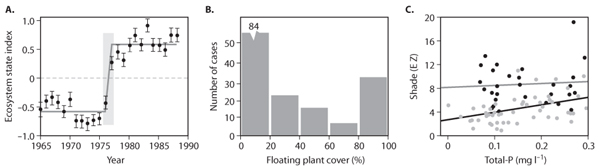
Figure 7. Three types of hints of the existence of alternative attractors from field data: (A) a shift in a time series, (B) multimodal distribution of states, and (C) dual relationship to a control factor. The specific examples are (A) a regime shift in the Pacific Ocean ecosystem (Modified with permission from Hare, S. R., and N. J. Mantua. 2000. Empirical evidence for North Pacific regime shifts in 1977 and 1989. Progress in Oceanography 47: 103–145); (B) bimodal frequency distribution of free-floating plants in a set of 158 Dutch ditches (Modified with permission from Scheffer, M., S. Szabo, A. Gragnani, E. H. van Nes, S. Rinaldi, N. Kautsky, J. Norberg, R.M.M. Roijackers, and R.J.M. Franken. 2003. Floating plant dominance as a stable state. Proceedings of the National Academy of Sciences U.S.A. 100: 4040–4045); and (C) different relationships between underwater shade and the total phosphorus concentration for shallow lakes dominated by Cyanobacteria (black circles) and lakes dominated by other algae (gray circles). (Modified with permission from Scheffer, M., S. Rinaldi, A. Gragnani, L. R. Mur, and E. H. Van Nes. 1997. On the dominance of filamentous cyanobacteria in shallow, turbid lakes. Ecology 78: 272–282)
In conclusion, one may obtain indications for the existence of alternative attractors from descriptive data, but the evidence can never be conclusive. There is always the possibility that discontinuities in time series or spatial patterns result from discontinuities in some environmental factor. Alternatively, the system might simply have a threshold response that is not related to alternative stability domains. The latter possibility is, of course, still very interesting. First, it helps to know that the system can change sharply if it is pushed across a threshold. Second, it often implies that under different conditions (as represented, for instance, by parameter 1 in figure 4), true alternative attractors could arise in the same system.
Experiments can be difficult to perform on relevant scales. However, they are much easier to interpret than field patterns. I discuss three major ways in which experiments can provide evidence for the existence of alternative attractors.
Different Initial States Lead to Different Final States
By definition, systems with more than one basin of attraction can converge to different attracting regimes depending on the initial state. In ecosystems, several sets of field observations suggest such so-called path dependency. For instance, similar excavated gravel pit lakes in the same area of the United Kingdom stabilized in either a clear or a turbid state in which they persisted for decades depending on the excavation method. Wet excavation created initially murky conditions and left the lakes turbid. By contrast, if the water was pumped out during excavation and the lake was allowed to refill only afterward, the initial state was one of clear water, and such lakes tended to remain clear over the subsequent decades. As always, there might be various alternative explanations for convergence to different endpoints.
However, path dependency can well be explored experimentally. The requirement is that one can study a set of replicates of a system that start their development from slightly different states and follow their evolution over time. An example is a study on the competition between floating and submerged aquatic plants (figure 8A). The development in a series of buckets incubated with different initial densities of the two plant types was followed. Although the set of initial states represented a gradual range of plant densities, all buckets developed toward dominance by one of the two types, indicating that the mix of the two types was unstable and that dominance by either of the two species represented alternative stable states. Another example of the experimental detection of path dependency comes from a study of plankton communities in small aquaria. Here it was shown that different orders of colonization from a common species pool may result in alternative endpoint communities, which are all stable in the sense that they are resistant against colonization by other species from the pool.
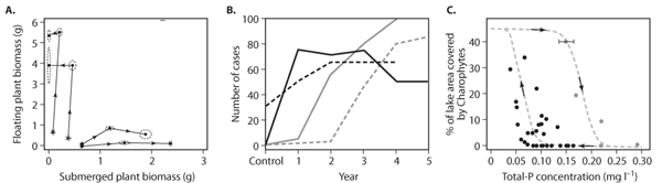
Figure 8. Three types of experimental evidence for alternative attractors: (A) different initial states leading to different final states, (B) disturbance triggering a shift to another permanent state, and (C) hysteresis in response to forward and backward change in conditions. Specific examples are the following: (A) path dependency in growth trajectories from competition experiments of a submerged plant (Elodea) and a floating plant (Lemna), which tend to different final states depending on the initial plant densities (Reproduced with permission from Scheffer, M., S. Szabo, A. Gragnani, E. H. van Nes, S. Rinaldi, N. Kautsky, J. Norberg, R.M.M. Roijackers, and R.J.M. Franken. 2003. Floating plant dominance as a stable state. Proceedings of the National Academy of Sciences U.S.A. 100: 4040–4045); (B) shifts of different shallow lakes to a vegetation-dominated state triggered by temporary reduction of the fish stock (Modified with permission from Meijer, M. L., E. Jeppesen, E. Van Donk, B. Moss, M. Scheffer, E.H.R.R. Lammens, E. H. Van Nes, J. A. Berkum, G. J. De Jong, B. A. Faafeng, and J. P. Jensen. 1994. Long-term responses to fish-stock reduction in small shallow lakes—interpretation of five-year results of four biomanipulation cases in the Netherlands and Denmark. Hydrobiologia 276: 457–466); and (C) hysteresis in the response of charophyte vegetation in the shallow Lake Veluwe to an increase and subsequent decrease in the phosphorus concentration. (Modified with permission from Meijer, M. L. 2000. Biomanipulation in the Netherlands—15 Years of Experience. Wageningen, the Netherlands: Wageningen University)
Disturbance Can Trigger a Shift to Another Permanent State
Another feature of systems with alternative attractors that can be tested experimentally is the phenomenon that a single stochastic event might push the system to another basin of attraction where it converges to an alternative persistent regime (figure 8B). This is often more practical in a real-life situation than trying to set a large set of “replicate” systems to a slightly different initial condition. As mentioned earlier, a good example from ecosystem management is that a temporary drastic reduction in the fish stock (biomanipulation) can move lakes from a turbid state to a stable clear condition. Lasting effects of single disturbances have also been studied in ecotoxicological research, where the inability of the system to recover to the original state after a brief toxic shock has been referred to as community conditioning. Such experiments should be interpreted cautiously. If one wants to demonstrate that the new state is stable, the return of the original species should not be prevented by isolation. Another problem is the potentially long return time to equilibrium, which may suggest an alternative stable regime even if it is just a transitional phase. For instance, biomanipulated lakes may remain clear and vegetated for years until they start slipping back to the turbid state.
Hysteresis in Response to Forward and Backward Change in Conditions
Demonstration of a full hysteresis in response to slow increase and subsequent decrease in a control factor also comes close to proving the existence of alternative attractors (figure 8C). Examples of hysteresis are seen in lakes recovering from acidification or eutrophication and in hemlock–hardwood forests responding to change in disturbance intensity. However, a hysteretic pattern may not indicate alternative attractors if the response of the system is not fast enough relative to the rate of change in the control factor. Indeed, one will always see some hysteresis-like pattern unless the system response is much faster than the change in the control variable.
In conclusion, experiments are potentially a powerful way to test whether a system may have alternative attractors, but there are important limitations to exploring large spatial scales and long time spans.
In summary, there is no silver-bullet approach to find out if a system has alternative basins of attraction separated by critical thresholds. Observations of sudden shifts, sharp boundaries, and bimodal frequency distributions are suggestive but may have other causes. Experiments that demonstrate hallmarks such as “path dependency” and hysteresis are much more powerful but can only be done on small, fast systems. Models that formalize mechanistic insights are essential to help improve our understanding of complex systems but remain difficult to validate. Clearly, our best approach is to build a case carefully, using all possible complementary approaches, and interpret the results wisely.
There are two ways in which insight into possible alternative stable states is useful when it comes to management of ecosystems. First, we try to manage the ecosystem in such a way that the risk of collapsing into another unwanted state is reduced. Equally important, and certainly more rewarding at first sight, is the possibility of using the insight for novel approaches to restoration, invoking a shift from an unwanted into a preferred alternative state.
From a management point of view, a crucially important phenomenon in systems with multiple stable states is that gradually changing conditions may have little effect on the state of the system but nevertheless reduce the size of the attraction basin (figure 3). This loss of resilience makes the system more fragile in the sense that it can easily be tipped into a contrasting state by stochastic events. This is also one of the most counterintuitive aspects. Whenever a large transition occurs, the cause is usually sought in events that might have caused it: The collapse of some ancient cultures may have been caused by droughts. A lake may have been pushed to a turbid state by a hurricane, and a meteor is thought to have dealt with the dinosaurs, leading to the rise of mammals. The idea that systems can become fragile in an invisible way as a result of gradual trends in climate, pollution, land cover, or exploitation pressure may seem counterintuitive. However, intuition can be a bad guide, and this is precisely where good and transparent systems theory can become useful. Resilience can often be managed better than the occurrence of stochastic perturbations. For instance, a lake that is not loaded with nutrients is less likely to shift to a turbid state in a climatically extreme year than a lake that has a near-critical concentration of nutrients. We cannot prevent heat waves or storms, but we can manage the long-term trends in pollution and nutrient load.
Finding smart ways to promote a self-propagating runaway shift from a deteriorated state to a good state is perhaps the most rewarding part of the work on alternative stable states in ecosystems. What is rewarding is that the transition can be relatively easy once you find the Achilles’ heel of the system. In its most elegant form, this is the sequence: Determine how to reduce the resilience of the bad state first and then reverse it with little effort at all. Biomanipulation, as a shock therapy to make turbid lakes clear again is a classic example of this approach. First, the resilience of the turbid state is reduced (and that of the clear state enhanced) by decreasing the nutrient load to the lake. Subsequently, a brief intensive fishing effort converts the system into the clear state.
An innovative idea related to managing ecosystems with alternative stable states is that we can often make smart use of natural variation in resilience. Recognizing this is important in strategies for promoting wanted transitions as well as for preventing unwanted transitions. Natural swings may open windows of opportunity to induce a transition out of an unwanted state. For instance, a rainy El Niño year may be a window of opportunity for forest restoration, and a year with low water levels may make it easier to push a shallow lake to the clear state. The other side of the coin is that natural swings can lead to situations in which resilience of a wanted state becomes dangerously small. Rangeland managers in Australia are already advised to anticipate droughts that hit the continent during El Niño years by reducing livestock to prevent potentially irreversible degradation of the land that may easily result from overgrazing in such years. Although, I know of few other examples, one can imagine that management directed at the prevention of bad transitions in periods with naturally low resilience could be useful in other fields. For instance, rainy years may lead to higher phosphorus loading and elevated water levels that reduce resilience of the clear state of a shallow lake. Mowing of submerged vegetation that would normally have little effect could induce a shift to the turbid state in such a year. Similarly, natural changes in marine circulation patterns can alter temperature and food supply in such a way that stocks of commercially important fish species become less resilient to fishing. For instance, cod is restricted to relatively cold water. This may well imply that recruitment is less successful in populations that live at the edge of the species range as well as in years when the temperature of the water in the region is elevated. Ideally, fishing pressure should thus be tuned to such marine regime shifts if collapse of the population is to be prevented, and we want to harvest most in years when this would not harm the system too much. Such smart adaptive management approaches that use insight in natural swings in resilience seem quite rare so far.
Carpenter, S. R. 2002. Regime Shifts in Lake Ecosystems: Pattern and Variation. Oldendorf/Luhe, Germany: Ecology Institute. Using lakes as an example, the author discusses various aspects of regime shifts. Particular attention is given to stochastic aspects and statistical problems of identifying regime shifts and alternative stable states.
Folke, C., S. Carpenter, B. Walker, M. Scheffer, T. Elmqvist, L. Gunderson, and C. S. Holling. 2004. Regime shifts, resilience, and biodiversity in ecosystem management. Annual Review of Ecology Evolution and Systematics 35: 557–581. This is an overview of current thinking about resilience of ecosystems written on the occasion of the 30th anniversary of the influential review by C. S. Holling in 1973.
Holmgren, M., and M. Scheffer. 2001. El Niño as a window of opportunity for the restoration of degraded arid ecosystems. Ecosystems 4: 151–159. This article presents an explanation of how reduced resilience during rainy years may be used to change barren semiarid regions back into a forested state by excluding grazers temporarily.
Scheffer, M. 2008. Critical Transitions in Nature and Society. Princeton, NJ: Princeton University Press. This book elaborates on the issues I cover in this chapter and also reviews case studies ranging from the climate system and ecosystems to socioeconomic dynamics.
Scheffer, M., and S. R. Carpenter. 2003. Catastrophic regime shifts in ecosystems: Linking theory to observation. Trends in Ecology and Evolution 18: 648–656. This article reviews how evidence for alternative stable states in ecosystems may be obtained.
Scheffer, M., S. R. Carpenter, J. A. Foley, C. Folke, and B. Walker. 2001. Catastrophic shifts in ecosystems. Nature 413: 591–596. This article reviews theory and examples of catastrophic shifts in ecosystems.