CHAPTER 7

Glacial-Interglacial Contrast

In the early 1970s, a meeting was held at GFDL to explore possible collaboration between climate modelers and paleoclimatologists. This was a time when a consortium of earth scientists had undertaken an ambitious project to reconstruct the state of the Earth’s surface at the last glacial maximum (LGM), which occurred approximately 21,000 years ago. At the meeting, John Imbrie of Brown University, one of the leaders of this project, convinced Manabe that the climates of the geologic past would be one of the most promising avenues of research for climate modelers. Their conversation began a long-term research project that continued during much of Manabe’s research career. In the early 1980s, Broccoli joined his group after graduate school at Rutgers University and began some of the modeling studies of glacial climate that will be presented in this chapter.

Paleoclimatologists and paleoceanographers have devoted a great deal of effort to reconstructing of the states of the ocean, land surface, and atmosphere at the LGM based upon the analysis of sediments from oceans and lakes, air bubbles trapped in ice cores, and other geologic signatures. Given the glacial-interglacial difference in surface temperature, continental ice sheets, and concentrations of greenhouse gases, attempts have been made to estimate the sensitivity of climate using climate models. In this chapter, we shall describe some of these attempts, searching for the most likely value of climate sensitivity.

The Geologic Signature

In the early 1970s, Imbrie and Kipp (1971) published a study that opened the way for the quantitative analysis of LGM climate. Using multiple regression analysis to relate the taxonomic composition of planktonic biota in deep sea sediments to sea surface temperature (SST), they found a close relationship between these two variables. Applying the relationship thus obtained, it was possible to translate the abundances of different types of planktonic biota preserved in deep sea sediments into estimates of past SST. Encouraged by the very promising results obtained from this method, Imbrie and colleagues embarked upon the Climate: Long-range Investigation, Mapping, and Prediction Project (CLIMAP; CLIMAP Project members, 1976, 1981) in order to reconstruct the state of the Earth’s surface at the LGM.

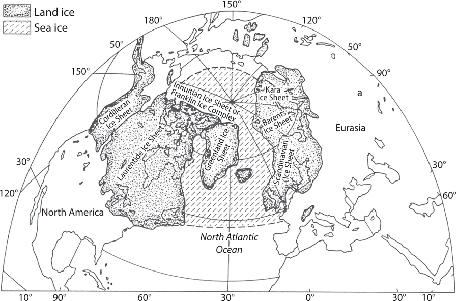
FIGURE 7.1 Distribution of continental ice sheets at the last glacial maximum. Modified from Denton and Hughes (1981).

The most dramatic features of the Earth at the LGM were the great ice sheets that covered large portions of Northern Hemisphere continents (figure 7.1). Although ice cover increased in many areas, the largest accumulation occurred in northeastern North America (Laurentide ice sheet) and northwestern Europe (Fennoscandian ice sheet), with smaller increases in western North America (Cordilleran ice sheet), European Russia, the Alps, the southern Andes, and West Antarctica.

One of the important products of CLIMAP is the reconstruction of these massive LGM ice sheets undertaken by Denton and Hughes (1981). Taking into consideration the outer margins of the ice sheets as indicated by geologic signatures such as moraines, they determined the shape of the ice sheets that would be in dynamic equilibrium. Over ice-free continental surfaces, CLIMAP reconstructed the distribution of vegetation at LGM from the taxonomic composition of pollen, using multiple regression analysis (Webb and Clark, 1977). The reconstructions of continental ice sheets and vegetation have been useful to climate modelers for determining the distribution of continental surface albedo during the LGM.

An important factor that influences the climate of the LGM is the concentration of atmospheric greenhouse gases such as carbon dioxide, methane, and nitrous oxide. The analysis of air bubbles found in ice cores reveals that the CO₂-equivalent concentration of these greenhouse gases at the LGM was about two-thirds of the preindustrial level (e.g., Chappellaz et al., 1993; Neftel et al., 1982), indicating that the greenhouse effect of the atmosphere was substantially smaller at the LGM than at present. Along with the massive continental ice sheets and extensive snow cover and sea ice that collectively reflect a large fraction of incoming solar radiation, the reduction of the concentration of greenhouse gases is also responsible for making the climate of the LGM much colder than the present. The reduction in greenhouse gases is particularly important in the Southern Hemisphere, where changes in albedo were not as extensive. Here we describe some of the early attempts to simulate the LGM climate using climate models and evaluate its implications for the sensitivity of climate.

Simulated Glacial-Interglacial Contrast

The first attempts to simulate the LGM climate using atmospheric GCMs were undertaken by Williams et al. (1974) and Gates (1976). These studies prescribed surface boundary conditions, including SSTs, based on geologic reconstructions of the LGM. Gates (1976) was the first to use the LGM distributions of SST, sea ice, and albedo of snow-free surface reconstructed by CLIMAP. In his study, the distribution of temperature at the continental surface was obtained as an output of the experiment. He found that the simulated temperature at many continental locations was broadly consistent with the temperature that CLIMAP estimated using various proxy data, such as the taxonomic composition of pollen in lake sediments (Webb and Clark, 1977). The agreement, however, does not necessarily imply that the model had realistic sensitivity, because surface temperature over the continents was closely constrained by prescribing the surface temperature of the surrounding oceans based on the CLIMAP reconstruction.

Hansen et al. (1984) conducted a similar numerical experiment using a version of the GISS atmospheric GCM. The distribution of seasonally varying SST in their control simulation was prescribed based upon modern observations. They also performed an LGM simulation using the LGM distribution of SST as reconstructed by CLIMAP, as Gates did in his study. They computed the difference in the net TOA flux of outgoing radiation between the two experiments and found that the heat loss from the net TOA flux is larger by about 1.6 W m⁻² in the LGM than the modern simulation. The excess heat loss indicated that the atmosphere-surface system of the model was attempting to cool further than the prescribed SST of LGM would allow. Hansen et al. interpreted this radiative imbalance as an indication either that their model was too sensitive (at ~4.2°C to CO₂ doubling) owing to overly large radiative feedback, or that the CLIMAP estimates of LGM SST used as a lower boundary condition were too warm.

The study of Hansen et al. attempted to infer the sensitivity of climate from the difference in the TOA flux of radiation between the two experiments, in which the LGM and modern distributions of SST were prescribed according to the CLIMAP reconstruction and modern observations, respectively. A more direct way to determine the climate sensitivity of a model would be to simulate the glacial-interglacial SST difference and compare it with the difference as determined by the CLIMAP reconstruction. The first attempt to pursue this approach was made by Manabe and Broccoli (1985). Here we describe the results they obtained and evaluate their implications for climate sensitivity.

The model used for their study was an atmosphere/mixed-layer-ocean model that was developed by Manabe and Stouffer (1980) as described in chapter 5. Two versions of this model were used. The fixed cloud (FC) version is the original version of the model, in which the distribution of cloud was prescribed and cloud feedback was absent. In the variable cloud (VC) version, the distribution of cloud was allowed to change and cloud feedback was in operation. These two versions of the model were originally constructed for the study of cloud feedback that was later published by Wetherald and Manabe (1988), as described in chapter 6. The sensitivity of the VC version to CO₂ doubling was 4°C and is much larger than the ~2°C sensitivity of the FC model. This large difference is attributable not only to the absence of cloud feedback in the FC version, but also to the difference in the strength of the sea ice albedo feedback in the Southern Hemisphere, where surface air temperature is substantially colder in the VC than in the FC version of the model. Irrespective of the specific causes of the difference in sensitivity, these two versions of the model were used in an effort to identify the sensitivity of climate that is more consistent with the glacial-interglacial difference in SST.

Manabe and Broccoli (1985) performed two sets of numerical experiments, using these two versions of the model. Each set of experiments included a present-day control run and a simulation of the LGM climate. All simulations started from an initial condition of an isothermal atmosphere at rest, but different boundary conditions were specified for the LGM and control simulations. In the LGM simulation, the atmospheric greenhouse gas concentration, surface elevation, and ice sheet and land-sea distributions were prescribed according to the ice core and CLIMAP reconstructions. (Changes in the Earth’s orbital parameters were not included, even though they have been identified as drivers of glacial-interglacial climate variations, because the parameters at the LGM happen to be similar to those of the present.) Owing in no small part to the absence of the large thermal inertia of the deep ocean below the mixed layer, it took only several decades for the model to closely approach a state of equilibrium. Throughout the course of the time integrations, the seasonal cycle of incoming solar radiation, the albedo of snow-free surface, and the CO₂-equivalent concentration of greenhouse gases were held fixed. The glacial-interglacial contrast of SST was then obtained as the difference between the simulated state of the LGM and that of the present.

Latitudinal profiles of the glacial-interglacial difference in zonal mean SST obtained from the FC and VC versions of the model (figure 7.2) can be compared with the zonal mean temperature difference obtained by CLIMAP. In this comparison, SST in ice-covered regions is defined as the temperature of the water at the bottom surface of the sea ice. Although the SST difference is larger in VC than FC at most latitudes, it is difficult to say which version of the model is closer to CLIMAP. This is because the difference between the CLIMAP reconstruction and either version of the model is much larger than the difference between the two versions of the model at many latitudes. For example, in low latitudes, the glacial-interglacial differences in SST obtained from both versions are substantially larger than the difference obtained by CLIMAP. In the middle latitudes of the both hemispheres, they are comparable in magnitude. In high latitudes of the Northern Hemisphere, poleward of 60° N, they are much smaller than the difference reconstructed by CLIMAP. Nevertheless, we found it encouraging that the latitudinal profiles of the glacial-interglacial SST difference obtained from the two versions of the model resemble broadly the profile obtained by CLIMAP.

Figure 7.3 illustrates schematically how the latitudinal profile of CLIMAP SST changes between the LGM and the present. As shown in figure 7.3a, the SST is relatively high in low latitudes at both the LGM and the present and decreases gradually with increasing latitudes up to the outer margin of sea ice, where it is at the freezing point of seawater (−2°C). The difference between the LGM and the present, shown in figure 7.3b, increases gradually with latitude, reaching a maximum at the LGM sea ice margin. Poleward of the LGM sea ice margin, the SST difference decreases sharply until it reaches zero over the high latitude ocean, which was covered by sea ice at the LGM and is also ice covered at present. The latitudinal profile of the glacial-interglacial SST difference described in this schematic resembles the profiles in figure 7.2, particularly in the Southern Hemisphere, where the distributions of SST and sea ice are more zonal than in the Northern Hemisphere.

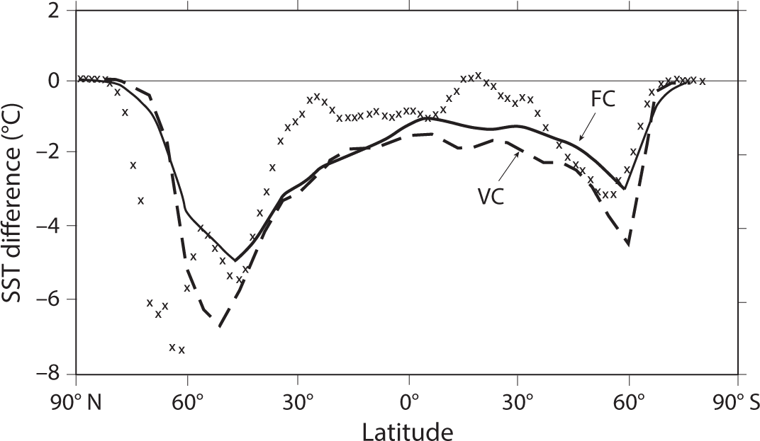
FIGURE 7.2 Latitudinal profiles of zonally averaged annual mean SST difference between the LGM and the present obtained from the FC and VC versions of the atmosphere/mixed-layer-ocean model. The crosses indicate the SST differences (average of January and July) obtained by CLIMAP. From Manabe and Broccoli (1985).

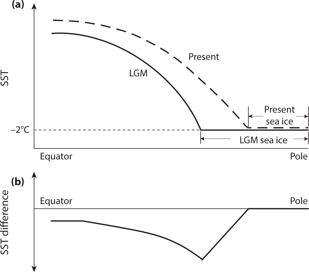
FIGURE 7.3 Schematic diagram illustrating (a) the correspondence between sea ice coverage and the latitudinal profile of SST at LGM and at present, and (b) the latitudinal profile of the glacial-interglacial SST difference (LGM − present).

In the numerical experiments performed here, the glacial-interglacial SST difference depends upon three factors: an expansion of continental ice sheets with high surface albedo, a reduction of CO₂-equivalent concentration of greenhouse gases, and an increase in the albedo of the snow-free surface. In order to evaluate the individual contributions of these changes to the glacial-interglacial difference in SST, Broccoli and Manabe (1987) performed additional numerical experiments using the FC version of the model. In each experiment, they changed one factor at a time, thereby evaluating the contribution of each change to the total glacial-interglacial SST difference.

Figure 7.4 illustrates the latitudinal distributions of the individual contributions obtained from this set of experiments. The expansion of the ice sheets has a large impact on SST in the Northern Hemisphere, whereas it is small in the Southern Hemisphere, where glacial-interglacial difference in continental ice extent is small. As noted by Manabe and Broccoli (1985), the damping of SST perturbation through interhemispheric heat exchange is much weaker than the in situ radiative damping in each hemisphere and has little effect upon the magnitude of the perturbation in middle and high latitudes. The effect of the lowered greenhouse gas concentrations is comparable in magnitude between the two hemispheres, though it is substantially larger in the Southern Hemisphere. The contribution from land albedo is relatively small in both hemispheres. Expressed in another way, the expanded ice sheets have the largest impact in the Northern Hemisphere, followed by the lowered concentration of greenhouse gases. In the Southern Hemisphere, on the other hand, the reduced greenhouse gas concentration is mainly responsible for the SST difference. Averaged over the entire globe, both expanded continental ice sheets and reduced greenhouse gases have a substantial impact on global mean SST, whereas changes in land albedo over ice-free areas have only a minor effect on a global basis.

The geographic distribution of the glacial-interglacial SST difference obtained from the VC version of the model is compared with the CLIMAP reconstruction in figure 7.5 as an example. In general, the model simulates reasonably well the broad-scale pattern of the SST difference. For example, regions of relatively large SST difference appear in the zonal belt of the Southern Ocean and in the northern North Atlantic Ocean, where the LGM sea ice margins are located, consistent with the schematic diagram shown in figure 7.3.

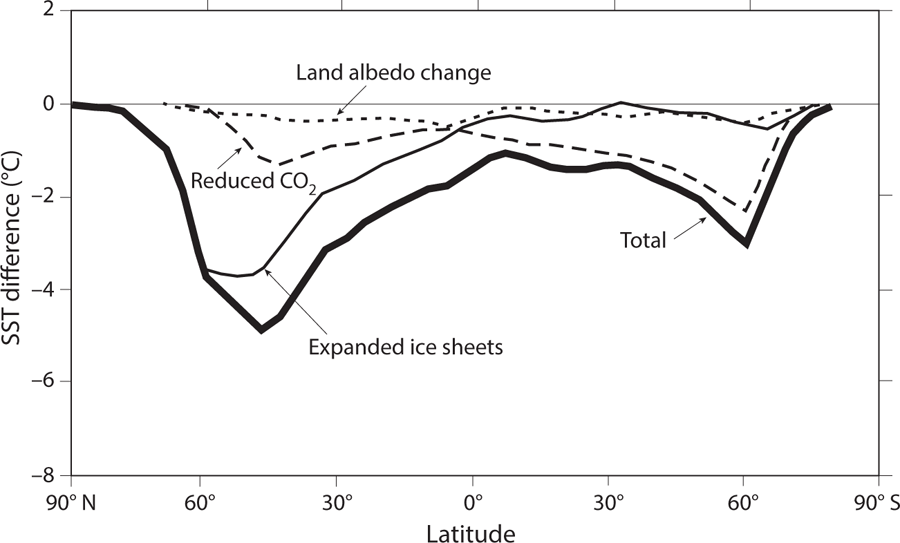
FIGURE 7.4 Latitudinal distributions of the individual contributions from expanded continental ice sheets, reduced atmospheric CO₂, and changes in albedo of ice-free land surface to the total glacial-interglacial SST difference (°C) obtained from the FC version of the atmosphere/mixed-layer-ocean model. From Broccoli and Manabe (1987).

Upon close inspection, however, one can identify many differences between the model simulation and the CLIMAP reconstruction. In the Southern Hemisphere, for example, the glacial-interglacial difference in SST is large in the zonal belt around 60° S in the model simulation, while it is large around 50° S in the CLIMAP reconstruction. In the northern North Atlantic, the SST difference is large in both the model simulation and the CLIMAP reconstruction. However, the area of large difference extends farther northward along the Scandinavian coast in the CLIMAP reconstruction. As shown schematically in figure 7.3, the glacial-interglacial SST difference reaches a maximum along the equatorward margin of sea ice at the LGM. Thus, it is likely that both of the discrepancies are at least partially attributable to the failure of the atmosphere/mixed-layer-ocean model used here to place realistically the location of the LGM sea ice margin.

In the CLIMAP reconstruction shown in figure 7.5b, the glacial-interglacial difference in SST has small positive values over extensive regions of the Pacific Ocean on both sides of the equator, suggesting that the sea surface was warmer at the LGM than at present in these regions. This reconstructed warming is quite counterintuitive and warrants close scrutiny. Examining the source of the data used by CLIMAP, Broccoli and Marciniak (1996) found that very few sediment core data are available in the regions of positive SST difference, and SST in these regions was often determined through subjective hand-contouring interpolation from the surrounding regions. Realizing that the SST difference obtained by CLIMAP may not be as reliable in these regions, they recomputed the zonal mean SST difference using the data only at those locations where sediment core data were available. In the tropical latitudes (30° N–30° S), the zonally averaged glacial-interglacial SST difference thus obtained is −1.8°C, which is much larger than the zonal mean SST difference of −0.6°C originally reconstructed by CLIMAP. It is, however, similar to the zonal mean temperature differences of −1.6°C and −2.0°C obtained from the FC and VC versions of the model, respectively.

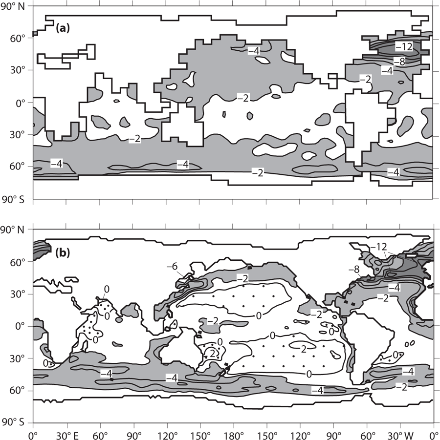
FIGURE 7.5 Geographic distribution of annual mean SST difference (°C) between the LGM and present (LGM − present): (a) SST difference obtained from the VC version of the model; (b) CLIMAP estimates (average of February and August). From Manabe and Broccoli (1985).

Since the publication of the CLIMAP study, many studies have suggested that tropical SST at the LGM was much lower than the CLIMAP reconstruction. For example, based upon the isotopic analysis of corals off Barbados, Guilderson et al. (1994) suggested that the tropical SST was colder by ~5°C than it is today. Beck et al. (1992) estimated tropical SST based upon the high positive correlation between SST and the strontium/calcium ratio in living corals. They found that the LGM tropical SST was colder than it is today by ~5°C, in agreement with the result obtained by Guilderson et al. These estimates of the tropical SST are much lower than the 1.8°C revised estimate of Broccoli and Marciniak.

On the other hand, Crowley (2000) found it very difficult to believe that tropical SST was so cold at LGM, wondering whether it would be possible for most corals to live in the tropical ocean at such low temperatures. He speculated that, if tropical SSTs were 5°C colder than the present, most corals would have been on the edge of or below the present level of habitability, and the taxonomic composition of plankton would have been quite different from what is indicated in the analysis conducted by CLIMAP. Therefore, he concluded that the SST difference between the LGM and present must be substantially less than the large values obtained by Guilderson et al. (1994) and Beck et al. (1992).

An alternative approach for the reconstruction of SST involves the use of alkenone molecules, which are produced by plankton and are preserved in marine sediments. For example, Brassell et al. (1986) found a strong correlation between temperature and the ratio of two types (diunsaturated and triunsaturated) of alkenone molecules. During the past few decades, many attempts have been made to estimate the glacial SST using the relationship between this ratio and SST. It appears that, in the coastal regions of the Atlantic and Indian oceans, where alkenone estimates were made, the modest reductions in SST reconstructed by this technique are not substantially different from those obtained by CLIMAP.

Improving the VC version of the model described above, Broccoli (2000) made a renewed attempt to simulate the distribution of SST at the LGM. The computational resolution of his model is twice as high as that of the FC or VC version of the model used for the study described above. In addition, he used the so-called Q-flux method, developed by Hansen and his collaborators at GISS, described in chapter 6. The application of this method allowed the geographic distributions of SST and sea ice in the control experiment to be more realistic than those obtained from either of the earlier FC or VC versions of the model. The sensitivity of this new version of the model was 3.2ºC, which is the median of the models evaluated for the IPCC Fifth Assessment Report (Flato et al., 2013).

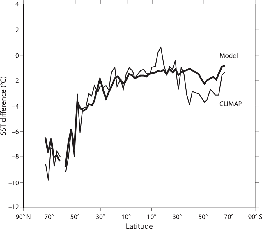
FIGURE 7.6 Latitudinal profiles of zonally averaged annual mean SST difference (°C) between LGM and present (LGM − present), from CLIMAP and the model of Broccoli (2000). Zonal averages were computed as the arithmetic average of SSTs at those locations where sediment-core data were available for CLIMAP. From Broccoli (2000).

Figure 7.6 compares the simulated and reconstructed profiles of the zonally averaged glacial-interglacial SST difference. Both profiles were determined using the SSTs from only those locations where CLIMAP sediment cores were available. As this figure shows, the agreement between the simulated and reconstructed profile is excellent, not only in the tropics but also in middle and high latitudes of the Northern Hemisphere. The agreement is also excellent up to ~35° S in the Southern Hemisphere. Poleward of 40° S, however, the SST difference simulated by the model is substantially smaller than the difference obtained from the CLIMAP sediment-core data. The discrepancy is the subject of further discussion in chapter 9, which evaluates the equilibrium response of the coupled atmosphere-ocean model to a reduction in the atmospheric concentration of CO₂. It suggests that the discrepancy is attributable to an absence of the interaction between the upper layer and the deep layer in the Southern Ocean of the atmosphere/mixed-layer-ocean model that Broccoli used in his study.

Given that the sensitivity of the model is 3.2°C, the similarity to the CLIMAP reconstruction would support the possibility that the sensitivity of the actual climate is not substantially different from 3°C. This result appears to be consistent with the results of Hansen et al. (1984) (discussed earlier in this chapter), which suggests that the actual sensitivity is likely to be less than the 4.2°C sensitivity of his model. Putting together the results obtained here with those from the preceding chapter, one can speculate that the sensitivity of the actual climate is likely to be about 3°C.

Developments in paleoceanography since the Broccoli study was completed at the turn of the millennium have led to additional approaches for estimating LGM SSTs. For example, the magnesium/calcium (Mg/Ca) ratio in shells of marine microorganisms has been used to estimate LGM tropical temperatures. Lea (2004) summarized results from a number of studies using Mg/Ca as well as alkenones to reconstruct SSTs, and concluded that tropical oceans cooled by 2.8°C ± 0.7°C at the LGM. Such cooling is somewhat larger than the CLIMAP estimates, but not as large as the early estimates from corals described previously. The Multiproxy Approach for the Reconstruction of the Glacial Ocean Surface project estimated an LGM reduction of tropical mean SST of 1.7°C (MARGO Project members, 2009), which is similar to the CLIMAP reconstruction as interpreted by Broccoli and Marciniak (1996). Annan and Hargreaves (2013) estimated a tropical SST cooling of 1.6°C ± 0.7°C.

These more recent reconstructions of tropical SST remain broadly consistent with a global climate sensitivity to CO₂ doubling of 3°C. A comprehensive analysis of reconstructions of past temperatures and radiative forcing from throughout Earth’s geologic history (PALAEOSENS Project members, 2012) estimated a range of 2.2°C–4.8°C for the actual climate sensitivity. Although the uncertainty associated with this estimate remains larger than would be desired, the sensitivity of the model employed by Broccoli (2000) lies close to the center of this range.