2

Mathematical Analysis

2.1  Fundamentals of Topology

This chapter aims to characterize what we mean by a ‘well-behaved’ feasible space and objective function. In order to do that, it introduces basic concepts of set theory and its applications to optimization.

As opposed to traditional textbooks in mathematics, the definitions herein provided do not follow a rigorous process and are intended to be as simple as possible to provide the engineer with a quick understanding of the concepts.

Additionally, this book provides examples from day-to-day practice of civil engineers in their professional activities. The reader should keep in mind that these examples will be revisited on more advance chapters.

2.1.1  Sets

A set is a group of elements that share at least one common characteristic. For instance, all members of the student association are part of a set, and their ‘membership’ is their common characteristic.

Subsets can be defined from a set; following the previous example, all freshmen (within the student association) are a subset of the previous set. Here, the reader realizes that it is convenient to give an easy-to-recall name to each set, so, for instance, the set of student members of the association can be called by the capital letter A, while freshmen could be called F. The indication that a set is part of a bigger set is given by F ⊂ A and reads F is a subset of A.

There are some classical sets widely used in all fields of knowledge and their letter-names are somewhat standard. For instance, all positive integer numbers called ‘natural’ are represented by N. All integers, whether positive or negative, are called by the letter Z; all rational numbers, that is, those defined as the ratio between two integers, are called by the letter Q. The rational numbers are classically defined as follows: $Q=x/x=\frac{p}{q},p,q\in Z,q\ne 0$.

As the reader can see, rational numbers can be defined replicating the previous definition with the addition of a constraint: the denominator cannot be zero, which makes sense, because otherwise the whole fraction will tend to infinity and infinity is undefined.

It should be noticed that Q does not comprise those numbers that failed to follow the previous definition. So any root that cannot be solved, and special numbers such as the base of natural logarithms, belong to the set called irrationals and are commonly represented by I. The union of irrationals and rationals, mathematically denoted as R ∪ I, creates the bigger set we all know as real numbers R (to distinguish from imaginary numbers).

A construction firm seeking to maximize their utility will define the space of possible profits as the natural numbers N because decimals are not relevant for managers, neither are negative amounts. However, a firm may well incur in losses; therefore, the definition may need to be revisited and changed to the set of integers.

In general, sets are used to either define the space at which a solution can be found, delimiting the alternatives to those that are relevant, or to characterize the elements that will be used in the analysis. For instance, when looking at traffic flows on a highway system, the engineer may want to delimit its analysis to only positive volumes of vehicles, and because we only care about complete vehicles, the space for the analysis will be composed of zero or positive integers.

If we look at all those ramps that enter a highway before a given control point, we can define a set of ramps R that are located before a given milepost.

2.1.2  Empty Set, Unions, Intersections, Complements

The empty set is the one containing no elements; however, it is still a set; you can think of it as the club where no one can satisfy its entry requirements and is denoted ∅. In the previous example, if we define a set composed by those highway ramps having more than 1900 vehicles/hour (veh/hour), and at the time no one satisfies this requirement, that is, every ramp observed is less than 1800 veh/hour, then there exists an empty set, which is denoted ∃ ∅.

Now let us create a group from those highways with high volume of traffic, such that peak hourly traffic flow is at least 1000 (veh/hour); if existing highway ramps are as given in Table 2.1, then the new set will have three elements A1, A4, A5, and we could denote this set by a letter, say H. A formal definition of these groups of highways with high volume is H : A1, A4, A5. We could create another set of ramps comprised of those with flow strictly smaller than 1000 veh/hour and call it L. Such set, L, is called the complement of H and is defined as the set of ramps that is not in H and is denoted H^c.

The union of H and L generates R and can be denoted HUL; notice the union is defined by the operator AND which means it is comprised of those elements that satisfy both the requirements of H and the requirements of L. In this case, the intersection of H and L has no elements, thereby satisfying the definition of ∅.

TABLE 2.1
Highway Ramps and Peak Traffic Volume

Ramp Number	Peak Traffic Flow	Flow Direction
A1	1100	Entry
A2	800	Entry
A3	600	Exit
A4	1300	Entry
A5	1800	Entry and exit
A6	900	Exit

2.1.3  Sets and Spaces

The distinction between a set and a space is given by the ability to measure a distance between any two elements of a set. Sets without this property cannot be defined as spaces. It is rather convenient to work with spaces.

However, in some cases, sets are composed of qualitative information, such as ranges of bearing capacity for the foundation soil (low, medium or high) or condition of road segments (good, fair, poor). In these cases, it is impossible to have a distance between what we call good road condition and fair road condition. Luckily often we have a numerical characterization, and instead of ranges of bearing capacity, we may have values of California bearing ratio (CBR) such as 80, 53 and 25.

In this case, it is simple and easy to know the distance as it is based on the absolute value of the subtraction |80 – 53|. In two or more dimensions, it is simply given by the norm, represented by the square root of the summation of the square of the differences, that is, $\sqrt[1/2]{{\left(x_i-y_i\right)}^2}$.

2.1.4  Upper and Lower Bounds

In defining civil engineering problems, it is important to be able to quickly realize if there is an upper (lower) bound for the problem at hand. Boundaries play an important role in warranting that the problem space is not undefined. The first thing we need to consider is if the space is ordered somehow, typically by the smaller < or bigger > operators.

Existence of a smaller (largest) element implies a lower boundary, but lack of it does not. Think, for instance, of the set F defined by the fractions of one divided by any positive integer, that is, $F=x/x=\frac{1}{q},q\in Z_{+},q\ne 0$; as the value of q increases, the value of the corresponding element in the set decreases and it is not possible to find a smallest element; however, zero is a lower boundary. Actually the set will approach zero asymptotically but never reach it. This leads us to the statement that if a set has a smallest element, it is unique.

In the context of highway ramps, traffic flow will define a space; as you can take the difference between any two values, it also has a lower limit as the minimum observed flow is zero vehicles per hour; however, does it have an upper limit?

At first glance, you may think that a highway can accommodate any number of vehicles and therefore there is no upper limit. However, as you will learn from your transportation classes, yes there is; typically, levels of service can go up to a maximum flow of about 1900 veh/hour per lane (called level of service E) and then decline as there is no sufficient space to accommodate more vehicles, thereby resulting in traffic jams.

Other examples of similar systems are given by infrastructure elements. Think, for per instance, of the flow of water on a storm sewer pipe. Is there a minimum value of flow? Yes zero, no rain! Is there a maximum flow? Yes, when the pipe is at full capacity (that is why there is flooding). Now let us move into a more interesting problem: imagine a landfill (garbage disposal facility). They are comprised of a piece of land, which is restricted in surface by its boundary limits and by volume to the maximum elevation that the local regulations and the maximum side slopes will allow you to rise the landfill hill. Is there a maximum capacity for a landfill? Yes, it is given by its volume, and the rate of arrival of garbage will determine how many days the landfill has left. Can I push the capacity beyond this upper limit? Only if you manage to alter its very definition, that is, purchase more land or change the regulations that limit it.

2.1.5  Open Balls, Open Sets, Closed Sets

In characterizing the feasible space, we need to identify upper and lower boundaries and to characterize the very fabric of the space itself. As it will soon become evident, these characterizations of the space require consideration of two concepts: closeness and compactness.

The need for defining a closed space is tied to the definition of compactness and both to the existence of a solution for an optimization problem.

Let us define a useful element called a ball. A ball in two dimensions is simply a circle centred at x₁ with radius r₁, and an open ball is the one that does not include its boundary.

An open set is the one for which I can always find an open ball, no matter how close I get to its limits. In other words, there is always an element q, q ≠ x₁ which is part of an open ball centred at any x₁ of the set, with some radius r₁. Notice that here the key is to take on small values of r₁ as one approaches the limit of the set.

For example, remember the case of F = 1/q, q ∈ Z₊, q ≠ 0; the set will be open at zero. In general, the definition of open set corresponds to the one that does not include its boundary, and therefore, there will always be an element between x₁ and the limit of the set (zero for the example).

One way to know if a set is closed is to check if its complement is open. Let us take an example: let us use the real numbers between one and five [1,5]. Is this an open set?, to answer it is take an open-ball centered at one, and use any radius, you will see that such ball irremediably reach beyond the limit of the set. In other words, there does not exist an element between the first value of the set and its limit; that is, in simple words, one can ‘walk’ on the edge of the set’s limit.

The problem with open sets is that one cannot reach their limit, and this creates an ill-defined problem because very often one desires to only consider solutions at the boundary of the feasible space as we will see in Chapter 3.

Hence, open intervals are open sets and closed intervals are closed sets. Another interesting definition is that of interior and boundary points, and more generally limit points. Let A ⊂ X and x ∈ X; then x is a limit point of A if every neighbourhood (open ball) of x intersects with A at a point other than x. In other words, p is a limit point of a space A if ∃ q ∈ A such that q ∈ B(p, r) for any r > 0. Start by moving a point x a bit є inside the space A.

It is easy to see that if the space is continuous, the intersection of any open ball centred at x with radius smaller than є will contain some points and help x satisfy the definition of a limit point. This kind of point is also an interior point.

If we return to the starting position and move x a bit є away but this time outside the region A, we can see that for open balls centred at this new location of x and with radius smaller than є the intersection of such open ball and the space A is empty.

So any interior point or boundary point is a limit point if A is closed. In practical terms, the definition of such points helps us identify the portions of the space we can work with (feasible space). But if A is open, the points at its boundary will not be elements of A; still they are limit points.

Notice the definition of a limit point does not require the limit point to be also part of the space. Hence, a closed space contains all its limit points. An open space will not. This simple definition will be very useful for quickly identifying the continuity and differentiability nature of some problems.

Let us look at some examples. Imagine we define the space for the amount of contracts a company may take to construct bridges in Canada. It turns out that such construction company can take on the construction of 1, 2, 3, …, n bridges but not on the construction of 0.1238765392 of a bridge, which would be catastrophic as the company’s reputation will indicate they barely did some work. When making decisions, this company will know that its decision variable is the number of bridges they will construct per year. Hence, the space A for bridge construction is given by integers.

Even though this observation appears trivial, it is not when solving for an optimization problem in which the levels of several decision variables must be chosen. Think of it as what makes a bridge: a superstructure, a substructure and a deck!, and in turn the deck requires materials (formwork, concrete, steel) in addition to the use of machinery and labour.

So the choice of constructing a bridge implies the use of other resources which are limited. Is the space of concrete continuous? It appears yes; we could select any amount of concrete measured in weight or volume. Is the space of labour continuous? Is it that of machinery?

Let us imagine now that we can break down everything in unitary terms and say that each linear meter of a 2-lane bridge requires 200 m³ of concrete, 50 steel rebars type 40M, 100 m² of formwork, 10 hours of machinery work and 5 people for 20 hours. Can you tell if the space of labour is closed?

It turns out that it is preferable to work with closed spaces because one can take any value within the space. The problem of an open space is that values at the boundary cannot be used; it is like seeing the $100 bill on the floor and not being able to grab it.

An example of an open space would be that of the maximum number of revolutions on your car dial; it is there, you can see it, but I really do not advice you to go there. Luckily, most of the cases will involve closed spaces.

2.1.6  Compactness

There exist several definitions of compactness. For the purpose of this book, I will limit compactness to the most simple one. A space is compact if it is both closed and bounded. This is known as the Heine–Borel definition.

A compact space corresponds to a feasible space that is ‘well behaved’. Hence, in order to have a well-behaved optimization problem, we require a compact space and a ‘well-behaved’ objective function.

Defining a decision variable (control variable) is an intrinsic requisite of having a compact space. Decision variables need to be characterized in terms of their membership to either the real, natural or integer numbers.

2.1.7  Convexity

A space is convex if for every pair of points within the object, every point on the straight-line segment that joins the pair of points is also within the space. For example, a solid cube is convex, but anything that is hollow or has a dent in it is not.

A function defined on an interval is called convex if the line connecting any two points on the graph of the function lies above the graph (plot) of the function. It is very important to quickly visualize convexity. The idea of convexity is particularly useful in unbounded problems because a solution may exist when the objective function is convex and the feasible space is concave. Concave simply follows the contrary; any line connecting any two points on the graph of the function lies below the graph (plot) of the function.

2.1.8  Plotting Objects

As you can see, the ability to graph objects on space becomes very useful when dealing with open, bounded, convex and continuity concepts. The ability to plot any given function is particularly useful for quick visualization.

This section provides the reader with the steps required to plot on MATLAB^®. I will look at two specific examples. The reader can possibly find more examples online. MATLAB contains three main windows: the history window, the command window and the workspace.

The workspace is commonly used for the definition of subroutines, we will not use it in this book. The command history keeps track of the commands you have used. The command window is where we input the commands I will cover in the following.

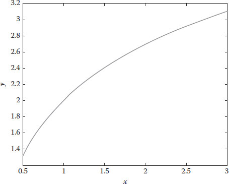
Let us take as first example plotting of the following function: y = 2 + log(x).

First, you need to define the range for any variable. On the command window, type x = 0.5 : 0.01 : 3; this will define the variable x starting at 0.5 ending at 3, with increments of 0.01.

Second, you need to define the function y, so type on the command window y = 2 + log(x).

Third, you can plot now, so type on the command window plot(x,y) and hit enter. You will obtain a graph.

Four, if you want to add a title for the graph, so type on the command window title(‘Plot of y versus x’), xlabel(‘x’), ylabel(‘y’) and hit enter. You will obtain the graph shown in Figure 2.1.

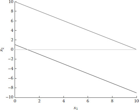
To clear the command window, type clc; to clear the variables, type clear. Now let us plot several lines into the same graph; presume you have the following feasible space defined by the following set of equations:

$\begin{array}{l}{x}_1+x_2\ge 1\text{,}\\ x_1\ge 0,x_2\ge 0\\ \text{and}\\ x_1+x_2\le 10\end{array}$

We define first the range for x₁ and x₂; as you can see, they go from zero to any number, but for practical purposes, we will define them up to a value of 11 given that there is a line crossing at an intercept of 10 with both axes. So we type on the command window x₁ = 1 : 11 and hit enter, then x₂ = 1 : 11 and hit enter.

The first equation needs to be expressed in terms of x₂, so it becomes x₂ = 1 − x₁; in MATLAB, we type x₂ = 1 − x₁. For the third equation, we need to create a new variable to store the relationship; we call it x₃ and type x₃ = 10 − x₁; as you can see, I have defined everything in terms of x₁. For the second equation, you already defined x₁ = 1:10; now you need to define the line that corresponds to zero, so you type a new variable, say x₄, and you type x₄ = 0 ∗ x₁.

FIGURE 2.1
MATLAB^® plot of y versus x.

On MATLAB, we need to indicate in the software the need to plot everything on the same graph; for this purpose, we use the command hold on. Here are the MATLAB commands in the required sequence to produce the graph:

x₁ = 1 : 10

x₂ = 1 − x₁

x₃ = 10x₁

x₄ = 0 ∗ x₁

hold on; plot(x₁, x₂, ‘r’); plot(x₁, x₃, ‘b’); plot(x₁, x₄, ‘g’); hold off.

After this, you produce the following graph. Notice that the code ‘r’ stands for red color line, ‘b’ stands for blue and ‘g’ stands for green. You can alternatively define labels and title using title(‘Plot of Feasible space’), xlabel(‘x₁’), ylabel(‘x₂’). Figure 2.2 shows the end result.

FIGURE 2.2
MATLAB plot of the feasible space.

2.2  Characterizing an Objective Function

A well-behaved objective function is continuous and differentiable. A function is continuous if for every open space in y the inverse image is an open space in x. This concept relies on the ability to have an inverse and for the purpose of this book can be simplified as the ability to map from any value in y to x. Inverse images of open sets are open. Picture a parabola and take any open space (i.e. on the y-axis, select an open interval). If the function is continuous, the inverse image will result in an open interval on the x-axis.

A function is continuous if for every convergent sequence with limit x the sequence converges to f(x).

Differentiability refers to the ability to take derivatives. For most of the problems studied in this book, we require a function to be twice differentiable, the first time to have first-order conditions. If a function is differentiable, then it is continuous.

2.2.1  Warranting Optimality

If a feasible space is compact and an objective function is continuous, then by Weierstrass theorem, the function attains a maximum and minimum on such space. This theorem is one of the battle horses of optimization and is the motivation behind careful definition of both feasible space and objective function.

Even though second-order conditions exist, I will deliberately ignore them in this textbook.

2.3  First-Order Conditions

You probably remember from your senior high school years that in your calculus class you learn something regarding how to find a maximum or a minimum.

First-order conditions refer to those regions of a function where the slope reaches a value of zero. The technique used to identify the point where the slope is zero is by taking the derivative of the function and making it equal to zero. This is however applicable to two-dimensional spaces.

For higher-dimensional spaces, we proceed in a similar way: we can take the partial derivative with respect to each variable and equalize it to zero.

The first-order condition can be used to identify the circumstances under which a certain variable can be optimized. If you are interested in finding out whether you reached a maximum or a minimum, then you may need to use the second derivative.

2.4  Lagrange Method

The Lagrange method is amply used in many fields. The method combines the objective with the constraints into one equation and uses first-order conditions to solve. Typically out of each first-order condition, you obtain one expression (equation) that gives you a representation of an optimal behaviour.

The Lagrange method can be summarized in the following steps:

1.  Write down your objective.

2.  Every constraint is multiplied by a parameter, the typical name for the parameters is lambda λ. If you have several constraints, then use one λ per constraint (λ_i). Sometimes, the time dimension may be present, then call the parameter ${\text{λ}}_i^t$ where i stands for the constraint and t for the time period. In the most general case, you could have one ${\text{λ}}_{i,j}^t$, where i is the decision variable, j is the individual for which we are solving and t is the period of time. We would not look at this level of detail; you could encounter this at recursive dynamic macroeconomic problems.

3.  Apply first-order condition; that is, take a partial derivative with respect to each decision variable and equal each to zero.

4.  Solve and obtain an expression for each decision variable.

Each optimization problem needs to be formulated as you saw in the previous chapter; the same is applicable here. Learning the mechanisms behind the nature of a problem is never easy; the more problems you formulate, the easier it will be to identify the bare bones of new problems. I will now introduce two examples—the formulation will be completely explained in the first one while in the second example the formulation will be given.

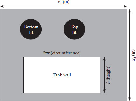
The first example is a very basic one. Consider a water tank of cylindrical dimensions given by a radius r for the bottom and a height h for the wall. The wall of the tank can be seen as a rectangle of dimensions 2πr. For the top and the bottom of the tank, you need circles. Figure 2.3 illustrates the initial set-up for the metal sheet cutting.

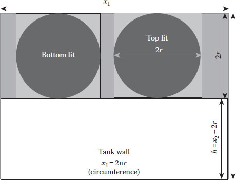
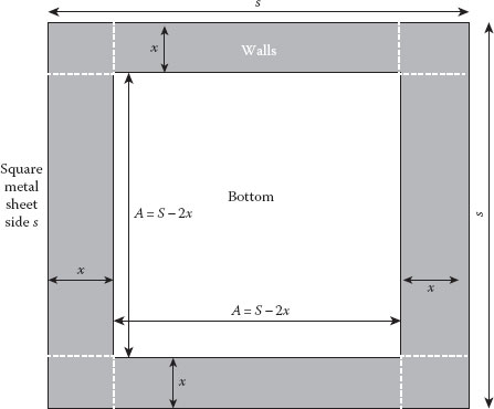
We will think of them as squares to simplify the process. The problem is how to maximize the volume of the tank while using a square sheet of metal to assemble it. Figure 2.4 illustrates the abstraction of the square metal for this problem. We start by placing two lids and a wall over the metal sheet.

FIGURE 2.3
Initial set for metal sheet.

FIGURE 2.4
Assuming squares for top and bottom.

The next thing you probably notice is that the squares needed for the bottom and top are of dimensions 2r. I have place them one next to the other one.

As you can see, I have written the height of the tank as a function of the radius and the given side size as x₂. We now try to formulate the objective: to maximize the volume. The volume is given by the tank height x₂ − 2r multiplied by the area of the bottom (and top, they are the same) given by π multiplied by r². The only decision variable in this optimization is the radius, so we want to find its value. The maximization takes the following form:

$(x_2-2r)(\text{π}{r}^2).$

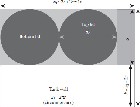
The constraints are shown in Figure 2.5; as you can see, we have one constraint per dimension of the metal sheet. For x₂, we know that it will be equal to h + 2r; however, we notice we do not know what h is, so it becomes a second decision variable. For x₁, we know that it has to be smaller or at most equal to 2r + 2r = 4r.

The final formulation is as shown in the following. We have one objective and two constraints.

$\underset{r}{\max }(x_2-2r)(\text{π}{r}^2).$

$\begin{array}{cc}{x}_1-2\text{π}r=0& x_2-2r-h\end{array}=0.$

FIGURE 2.5
Constraints on metal sheet.

We use the Lagrange method to solve. First, we create the Lagrangian, an equation that puts together both the objective and the constraints.

$L=\underset{r}{\max }(h)(\text{π}{r}^2)+{\text{λ}}_1(x_1-2\text{π}r)+{\text{λ}}_2(x_2-2r-h).$

Our objective is to estimate the values of the radius r and the height h in terms of x₁ and x₂. The next step in the Lagrange method (step 3) is to take partial derivatives with respect to each decision variable and with respect to each Lagrange multiplier and equal to zero. This corresponds to the following first-order conditions:

$\begin{array}{l}\frac{dL}{dr}=2\text{π}hr-4{\text{λ}}_1-2{\text{λ}}_2=0,\\ \frac{dL}{dh}=\text{π}{r}^2-{\text{λ}}_2=0,\\ \frac{dL}{d{\text{λ}}_1}=x_1-2\text{π}r=0,\\ \frac{dL}{d{\text{λ}}_2}=x_2-2r-h=0.\end{array}$

The last step (step 4) is to solve the system of equations and find the values of the decision variables (r and h in this case). We take the third equation and directly obtain the value for $r=\frac{x_1}{2\text{π}}$. We input this explicit value of r into the last equation and solve for h:

$\begin{array}{l}{x}_1-2\text{π}=0\\ r=\frac{x_1}{2\text{π}}\\ x_2-2r-h=0\\ x_2-2\left(\frac{x_1}{2\text{π}}\right)=h\\ x_2-\frac{x_1}{\text{π}}=h\end{array}$

The amounts x₁ and x₂ are given to you; they are the dimensions of the metal sheet. Therefore, the radius r of the bottom and top depends on x₁ and the height depends on both x₁ and x₂.

2.5  Gradient Search

The gradient search is a technique to find an optimal point. This technique follows an iterative process that changes the value of the variables until you are close enough to a maximum or a minimum given the satisfaction of the first-order condition.

This formulation of this technique can be explained using the Lagrange method.

The idea behind the gradient search is to find the optimal step size s to walk when trying to approach an optimal point. The discrete steps Δx and Δy taken in the x and y directions lead to a total change in the objective Δz which is approximately given by

$\text{Δ}z=\frac{\text{δ}z}{\text{δ}x}\text{Δ}x+\frac{\text{δ}z}{\text{δ}y}\text{Δ}y.$

The partial derivative is assessed at the current location c for both directions (x and y). The objective is constrained by Pythagoras as follows:

${(\text{Δ}x)}^2+{(\text{Δ}y)}^2={(s)}^2.$

This can be formulated using the Lagrange method, and our decision variables will be Δx and Δy. The Lagrangian is

$L=\frac{\text{δ}z}{\text{δ}x}\text{Δ}x+\frac{\text{δ}z}{\text{δ}y}\text{Δ}y+\text{λ}(s^2-\text{Δ}{x}^2-\text{Δ}{y}^2).$

Taking partial derivatives, we get the following:

$\begin{array}{lll}\frac{\text{δ}L}{\text{δ}\left(\text{Δ}x\right)}\hfill & =\hfill & \frac{\text{δ}z}{\text{δ}x}-2\text{λ}\text{Δ}x=0,\hfill \\ \frac{\text{δ}L}{\text{δ}\left(\text{Δ}y\right)}\hfill & =\hfill & \frac{\text{δ}z}{\text{δ}y}-2\text{λ}\text{Δ}y=0,\hfill \\ \frac{\text{δ}L}{\text{δ}\text{λ}}\hfill & =\hfill & (s^2-\text{Δ}{x}^2-\text{Δ}{y}^2)=0.\hfill \end{array}$

Solving for λ in the first two equations, we get the following:

$\begin{array}{lll}\text{λ}\hfill & =\hfill & \frac{1}{2\text{Δ}x}\frac{\text{δ}z}{\text{δ}x},\hfill \\ \text{λ}\hfill & =\hfill & \frac{1}{2\text{Δ}y}\frac{\text{δ}z}{\text{δ}y}.\hfill \end{array}$

Equal and solve

$\begin{array}{lll}\frac{1}{2\text{Δ}x}\frac{\text{δ}z}{\text{δ}x}\hfill & =\hfill & \frac{1}{2\text{Δ}y}\frac{\text{δ}z}{\text{δ}y},\hfill \\ \frac{\text{δ}z/\text{δ}x}{\text{δ}z/\text{δ}y}\text{Δ}y\hfill & =\hfill & \text{Δ}x.\hfill \end{array}$

Substituting into the step size equation given by Pythagoras, we find

$\frac{s\frac{\text{δ}z}{\text{δ}y}}{\sqrt{\frac{\text{δ}{z}^2}{\text{δ}y}+\frac{\text{δ}{z}^2}{\text{δ}x}}}=\text{Δ}y.$

Similarly,

$\frac{s\frac{\text{δ}z}{\text{δ}x}}{\sqrt{\frac{\text{δ}{z}^2}{\text{δ}y}+\frac{\text{δ}{z}^2}{\text{δ}x}}}=\text{Δ}x.$

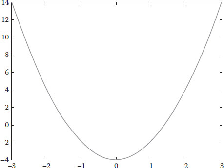
These two equations are written in terms of a step size s and the values of slopes at specific points; all values are known and the only unknown is the step size. You can take and test this value and monitor the value of the derivative until it approaches zero. Each time you move, you need to update the current value of $x_{i+1}=x_i+\text{Δ}x$ and of $y_{i+1}=y_i+\text{Δ}y$. Let us look at an example; consider the following equation: $Z=x^2+y^2-4$. This equation can be graphically represented by Figure 2.6.

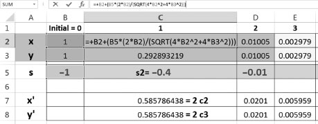
The gradient search method can be set up in Excel in order to estimate both the value of Δx and Δy and the corresponding value of the derivative (which hopefully will approach zero). Figure 2.7 shows a screenshot of the main interface created in Excel and the codes used to achieve both purposes mentioned previously.

FIGURE 2.6
Gradient example: graphical representation.

FIGURE 2.7
Excel spreadsheet for gradient search.

If we take partial derivative, it is easy to see that $\frac{\text{δ}z}{\text{δ}x}=2x$, which in Excel translates to 2C2 given that C2 is the corresponding cell with the current value for x.

Similarly for y, we obtain that the partial derivative is $\frac{\text{δ}z}{\text{δ}y}=2y$, which in Excel translates to 2C3 given that C3 is the corresponding cell with the current value for x.

The explicit forms for the Δx and Δy increments considering the previous derivative are the following:

$\frac{B5\ast \left(2\ast B2\right)}{\sqrt{4\ast B{2}^2+4\ast B{3}^2}}=\text{Δ}y$

and

$\frac{B5\ast \left(2\ast B3\right)}{\sqrt{4\ast B{2}^2+4\ast B{3}^2}}=\text{Δ}x.$

These equations are only measuring the differences, so they have to be added to the initial amounts at each step. This is achieved by simply adding at the beginning the initial amount as shown before and as shown by the Excel spreadsheet in Figure 2.7:

$x+\frac{B5\ast \left(2\ast B2\right)}{\sqrt{4\ast B{2}^2+4\ast B{3}^2}}=\text{Δ}x$

and

$y+\frac{B5\ast \left(2\ast B3\right)}{\sqrt{4\ast B{2}^2+4\ast B{3}^2}}=\text{Δ}y.$

Exercises

1.  Define the control variables in the following cases and identify the feasible space boundaries.

a.  Pipe to conduct rainwater

b.  Traffic flow of one lane at a given bridge

c.  Bearing soil capacity for the design of a foundation

d.  Concrete strength for the design of a column

e.  Water pressure on a system of water mains

2.  Characterize the objective function in the same circumstances as before with the following additional information.

FIGURE 2.8
Metal sheet for Exercise 3.

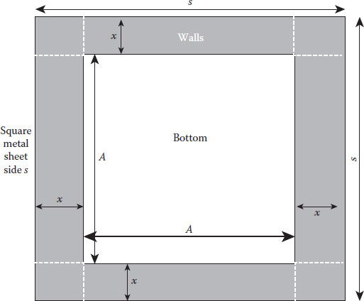
3.  Solve using the first-order condition (FOC) method. A parallelepiped water tank (think of a square-like section or a box) made out of a square metal sheet of side s as shown in Figure 2.8. The box has no lid (no top cover). Define the objective and constraints and solve using the FOC method.

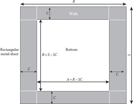
4.  Solve the following using the Lagrange method. Consider a parallelepiped water tank (think of a rectangular-like section) made out of a rectangular metal sheet as shown in Figure 2.9. The box has no lid (no top cover). Define the objective and constraints and obtain the derivatives of step 3 using the Lagrange method. Try to solve (hint: replacing the constraints into the objective gives you a fast-track way to solve).

5.  For the previous example, obtain an expression for the optimal area size for the bottom of the box. Formulate the objective (and constraints if necessary) and solve to find the optimal value of C to cut the metal sheet. Use this additional information to solve Problem 4.

6.  Formulate and solve the following problem.

A driver on a highway is using gravity; maximum speed on the highway is 100 km/h and, minimum speed is 60 km/h. The driver accelerates to about 140 km/h; then shifts from 6 to neutral (manual gear car) and lets the car roll/go downhill by gravity until friction slows down his car to about 80 km/h. By doing this, the car engine’s revolutions (cycles per second) drop from about 2.0 rpm to about 1.0 rpm, so fuel consumption drops by 50% during the time the car is in neutral.

FIGURE 2.9
Metal sheet for Exercise 4.

Assuming you are optimizing the driver behaviour, what is the minimum amount of time T1 the driver should go at 1.0 rpm in order to optimize saving. Assume $1 per minute is the average fuel saving when the vehicle goes at 1.0 rpm; let T1 be the amount of time the car goes at 1.0 rpm. Suppose the likelihood of getting a ticket of $220 is 1%, the likelihood of crashing for any reason is 0.1% and the mean estimated cost of crash is $2500. Let (T1/2)² be the amount of time the driver is going at a speed higher than the allowed, and therefore being exposed to a ticket or lacking proper control to avoid a collision.

Formulate the objective as maximization of savings, and formulate any constraints (if applicable) and solve using first-order condition.

7.  Identify the feasible space (defined by the constraints) and provide an explanation if the space is closed or open, and bounded:

a.  The feasible space is defined according to compliance with the following set of constraints: x₁ + x₂ ≥ 1, x₁ ≥ 0, x₂ ≥ 0 and x₁ + x₂ ≤ 10. Hint: Plot the constraints.

b.  The feasible space is defined according to compliance with the following set of constraints: x₁ + x₂ ≥ 1, x₁ ≥ 0, x₂ ≥ 0 and x₁ + x₂ ≤ 10. Hint: Plot the constraints.

c.  The feasible space is defined according to compliance with the following set of constraints: x₁ + x₂ > 1, x ≥ 0, x₂ ≥ 0 and x₁ + x₂ ≤ 10. Hint: Plot the constraints.

d.  The feasible space is defined according to compliance with the following set of constraints: x₁ + x₂ > 1, x₁ ≥ 0, x₂ ≥ 0. Hint: Plot the constraints.

e.  The feasible space is defined according to compliance with the following set of constraints: x₁ + x₂ > 1, x₁ ≥ 0, x₂ ≥ 0 and x₁ + x₂ ≥ 10. Hint: Plot the constraints.

f.  The feasible space is defined according to compliance with the following set of constraints: $x_1^2$ + $x_2^2$ ≤ 1, x₁ ≥ 0, x₂ ≥ 0. Hint: Plot the constraints.

g.  The feasible space is defined according to compliance with the following set of constraints: $x_1^2$ + $x_2^2$ ≥ 1, x₁ ≥ 0, x₂ ≥ 0 and x₁ + x₂ ≤ 10. Hint: Plot the constraints.

h.  The feasible space is defined according to compliance with the following set of constraints: $x_1^2$ + $x_2^2$ > 1, x₁ ≥ 0, x₂ ≥ 0 and x₁ + x₂ ≤ 10. Hint: Plot the constraints.

i.  The feasible space is defined according to compliance with the following set of constraints: $x_1^2$ + $x_2^2$ ≥ 1, x₁ > 0 and x₁ + x₂ ≤ 10. Hint: Plot the constraints.

8.  Identify in each of the previous cases where do you have a compact feasible space.

9.  The following are objective functions for each of the items under Problem 7. Identify if the objective is continuous, and then identify by Weierstrass theorem if there must be an optimal point (either minimum or maximum).

a.  $x_1+2x_2.$

b.  $x_1\text{ if }{x}_1<2\text{ and }{x}_1^2\text{ if }{x}_1\ge 2.$

c.  $x_1+3x_2\text{if}{x}_2<1\text{and}3x_1+x_2\text{if}{x}_2\ge 1.$

d.  $x_1+3x_2\text{if}{x}_2<1\text{and}3x_1+x_2\text{if}{x}_2\ge 2.$

e.  $2x_1+2x_2.$

f.  $x_1^2+x_2^2.$

10.  Identify if the space is convex:

a.  The feasible space is defined according to compliance with the following set of constraints: x₁ + x₂ ≥ 1, x₁ ≥ 0, x₂ ≥ 0, x₁ + x₂ ≤ 10. In addition, the space comprised between the following two lines must be removed from the feasible space x₁ + x₂ > 3 and x₁ + x₂ < 4.

b.  The feasible space is defined according to compliance with the following set of constraints: x₁ + x₂ ≤ 1, x₁ ≤ 0, x₂ ≤ 0and x₁ + x₂ ≥ 10. Hint: Plot the constraints.

c.  The feasible space is defined according to compliance with the following set of constraints: x₁ + x₂ ≥ 1, x₁ ≥ 0, x₂ ≥ 0and x₁ + x₂ ≤ 10. Hint: Plot the constraints.

d.  The feasible space is defined according to compliance with the following set of constraints: $x_1^2$ + $x_2^2$ ≤ 1, x₁ ≥ 0, x₂ ≥ 0. Hint: Plot the constraints.

e.  The feasible space is defined according to compliance with the following set of constraints: $x_1^2$ + $x_2^2$ ≤ 4 and $x_1^2$ + $x_2^2$ ≥ 1, x₁ ≥ 0, x₂ ≥ 0, x₁ + x₂ ≥ 10 and x₁ + x₂ ≤ 12. Hint: Plot the constraints.

Solutions

1.  a.  Decision variable = flow capacity on the pipe, space defined on positive real numbers. Lower boundary = zero, upper boundary = largest market-available pipe size.

b.  Decision variable = number of vehicles per hour per lane, space defined on positive integer numbers. Lower boundary = zero, upper boundary = commonly 1900 veh/hour/lane.

c.  Decision variable = foundation dimensions in centimetres, space defined on positive integer numbers (notice you would not design half a centimetre, and as a matter of fact, your design will be conditioned by rebar length in discrete jumps of dimensions). Lower boundary = zero, upper boundary = largest possible foundation size as restricted by neighbour properties or foundation budget.

d.  Decision variable = concrete strength, space defined on positive real numbers. Lower boundary = zero, upper boundary = largest market-available concrete strength. Notice in this case that concrete strength could take any value with decimals although the prescription when you buy goes on finite intervals.

2.  Objective is defined as

a.  The objective is to maximize pipe capacity.

b.  The objective is to maximize traffic flow (number of vehicles per hour).

c.  The objective is to maximize bearing capacity.

d.  The objective is to maximize concrete strength.

e.  The objective is to maximize water pressure.

3.  Figure 2.10 shows the relationships between the side size and the unknown amounts for the bottom side (A) and wall height (x).

The volume is $\underset{x}{\max }(S-2x)(x)$.

The partial derivative takes the form

$\frac{dL}{dx}=S-4x=0.$

FIGURE 2.10
Solution of Exercise 3.

From this, we see that x takes the value of $\frac{s}{4}$, and this will return in the optimal volume (maximum) for the water tank.

4.  In this case, you probably notice that x must be equal to y; in other cases, you would have an uneven wall height, so I will only use only x from now on. The volume is

$\underset{ABC}{\max }ABC.$

Subject to the following constraints:

$\begin{array}{l}S-2C-B=\mathrm{0,}\\ R-2C-A=0.\end{array}$

We create the Lagrangian:

$L=\underset{A,B,C}{\max }ABC+{\text{λ}}_1\left(S-2C-B\right)+{\text{λ}}_2\left(R-2C-A\right).$

Take partial derivatives with respect to each unknown (i.e. A, B, C) and the Lagrange multipliers:

$\begin{array}{lll}\frac{dL}{dA}\hfill & =\hfill & BC-{\text{λ}}_2=0,\hfill \\ \frac{dL}{dB}\hfill & =\hfill & AC-{\text{λ}}_1=0\hfill \\ \frac{dL}{dC}\hfill & =\hfill & AB-2{\text{λ}}_1-2{\text{λ}}_2=0\hfill \\ \frac{dL}{d{\text{λ}}_1}\hfill & =\hfill & S-2C-B=0,\hfill \\ \frac{dL}{d{\text{λ}}_2}\hfill & =\hfill & R-2C-A=0.\hfill \end{array}$

Remember that both R and S are given, which are the dimensions of the metal sheet used to create the water tank, we are interested in finding the values of A, B, C, not the value of the Lagrange multipliers. Unfortunately, we need to find these values to be able to solve.

$\begin{array}{l}BC-{\text{λ}}_2=0\text{ then }BC={\text{λ}}_2,\\ AC-{\text{λ}}_1=0\text{ then }AC={\text{λ}}_1.\end{array}$

We take the first equation and replace the Lagrange multipliers.

$\begin{array}{l}AB-2AC-2BC=0,\\ \frac{AB}{2}=C\left(A+B\right).\end{array}$

The last two equations tell us that if 2c = 2c, then

$S-B=2C$

and

$R-A=2\mathrm{C.}$

Therefore,

$S-B=R-A\text{ and }S-R=A+B.$

Given the fact that both S and R are known amounts, its difference is also a fixed known amount (such as 2, 7, 15, just to mention a few possibilities). So we end up with two equations that characterize the problem. The first one tells us the relationship between the metal sheet and the dimensions of the bottom of the box:

$B=\frac{S-R}{A}$

and correspondingly,

$A=\frac{S-R}{B}.$

The second one establishes the size of the wall in terms of the dimensions:

$C=\frac{AB}{2\left(A+B\right)}.$

5.  Figure 2.11 illustrates the solution for Exercise 5. The objective must consider two constraints: the first constraint is for the side A and is equal to R = A + 2C, the second constraint is for the other side B and is equal to S = B + 2C. We input this constraint directly into the equation for maximum area, which simply multiply both dimensions. We use the FOC to solve.

FIGURE 2.11
Solution of Exercise 5.

$\begin{array}{l}L=\underset{C}{\max }(R-2C)(S-2C),\\ L=\underset{C}{\max }RS-2CR-2CS+4C^2.\end{array}$

This simpler form allows us to handle one decision variable C and solve for it.

$\frac{dL}{dC}=-2R-2S+8C=0.$

We find that −2R − 2S + 8C = 0 leads us to (R + S)/4 = C. Both values R and S are known, so C is known. This result can be used back in Question 4 to find an expression for the optimal volume.

Recall that

$S-B=2C$

and

$R-A=2C.$

Knowing that

$C=\frac{R+S}{2},$

then

$S-B=\frac{R+S}{2}$

which means that

$S-\frac{R+S}{2}=B.$

Similarly,

$R-\frac{R+S}{2}=A.$

6.  The cost can be expressed as (220 * 0.01 + 2500 * 0.001). This cost is applicable only when the driver is exceeding the maximum allowable speed. That fraction of the total time is given by $\frac{T{1}^2}{2}$. The objective would then be

$\underset{T1}{\max }T1-\frac{T{1}^2}{2}\left(220\ast 0.01+2500\ast 0.001\right).$

Take a partial derivative with respect to t1 and equal to zero.

$1-T1(4.7)=0\text{ which results in }T1=1/4.7=\mathrm{0.2127.}$

This means that the optimal amount of time to exceed the speed is 21.27% of the time.

7.  It is open when the inequality does not include the equal: that is, it uses either smaller or bigger, and the side in consideration is part of the boundary of the feasible space.

It is unbounded when it misses one portion of the boundary. The following are the answers for each subitem of Question 6.

a.  Closed and bounded.

b.  Open and bounded.

c.  Open and bounded.

d.  Open and unbounded.

e.  Closed and bounded. Is one quarter of a circle on quadrant I.

f.  Closed and bounded. Is one quarter of a circle as bottom and line as top.

g.  Open and bounded. Is one quarter of a circle as bottom and line as top.

h.  Open and unbounded.

i.  Closed and bounded.

8.  The answer for Question 8 is

a.  Compact

b.  Noncompact

c.  Noncompact

d.  Noncompact

e.  Compact

f.  Compact

g.  Noncompact

h.  Noncompact

i.  Compact

9.  Objectives defined by multiple segments could imply discontinuities, however, in some cases the function may still be continuous. Let us look at the answers item by item.

a.  Continuous, and yes Weierstrass warrants optimality.

b.  Discontinuous.

c.  Continuous, with change of slope; yes Weierstrass warrants optimality.

d.  Discontinuous with missing segment.

e.  Continuous; you have a straight line; yes Weierstrass warrants optimality.

f.  Continuous; you have a circle again; yes Weierstrass warrants optimality.

10.  Anywhere we have a hole or missing portion, there would be problems with convexity. Let us look at the case-by-case answers:

a.  It is not convex; there is a hole (rectangular wedge missing).

b.  It is not convex; the constraints actually define the hole inside and the feasible space outside.

c.  It is convex.

d.  It is convex.

e.  It is not convex; there are two well-identified portions of the feasible space: one goes between two portions of a quarter of a circle and the other between two straight lines.