7

Transport and Municipal Engineering

7.1  Introduction

This chapter introduces the reader to several classical problems related to transportation systems analysis. Some of these classical problems serve to develop a foundation for more sophisticated problems closer to those faced in real life. Several simplifications serve to facilitate the formulation, and as we advance, more elements will be brought into the model. The problems will take advantage of methods learnt in previous chapters using tools readily available in Excel. More advanced and complex problems may need to be solved elsewhere.

7.2  Location of a Facility within an Area

How can planners at a municipality (or government body) choose the best location for a facility that must provide service to the public at large? You can think of a health clinic, a fire station, ambulance or any other emergency response unit. On a larger scale, you can even think of a regional park, a land field, an airport, an intermodal station, a library or even a market.

Two main indicators are important for this problem: travel time between all pairs of user location and the facility and the overall cost. Often, we engineers must attempt to reduce to a minimum the number of facilities but guarantee a sufficient coverage. For instance, you may want to build a health clinic that anybody can reach in 15 minutes or less or a fire station that can reach help to any location in town in no more than 10 minutes.

Sometimes, this task is impossible, and a single station cannot deliver the expected service on time. In such cases, two or more facilities would be needed. Having two facilities opens a new dimension to this problem; we will call it ‘coverage’. Coverage relates to the ability to have as many duplications as possible, that is, we will locate the emergency response unit in such a way that it maximizes coverage in addition to minimizing total network travel time and cost.

FIGURE 7.1
Handmade node structure.

Let’s look at the first example. Suppose we have to find the best location for a police station. Presume for the first formulation that one police station is enough, and we will only attempt to minimize total network travel time between the police station and the different neighbourhoods.

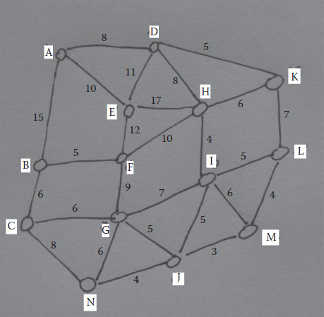
A simplified way to solve the problem is by taking a representation of the city based on its road network (links) and its neighbourhoods (nodes). Simply take a piece of paper and prepare a drawing like the one shown in Figure 7.1.

Even though nodes should carry the name of places, we have numbered them for convenience. The links do not necessarily represent actual roads; rather, they serve to connect neighbourhoods. Additionally, links are presumed to serve traffic moving in both directions; in some cases, we could restrict it to one direction of movement, and this would be represented by an arrow.

When assembling this type of problems, the municipal engineer needs to obtain a good estimation of the travel time, which can be initially based on field observations, but he or she must bear in mind that the travel time changes throughout the day, as congestion increases during morning, midday and evening peak hours (when most of the commuting from/to work occurs).

Travel time (in minutes) and possible directional restrictions (arrows) had been added to our example (Figure 7.1). Remember, many other variables could influence the travel time, for instance, surface type (gravel or paved), road condition (potholes will slow you down), alignment adequacy (unnecessarily curvy roads), type of terrain (rolling, mountainous) and intersections. We will further elaborate this in Chapter 8 when a framework to prioritize infrastructure decisions is proposed.

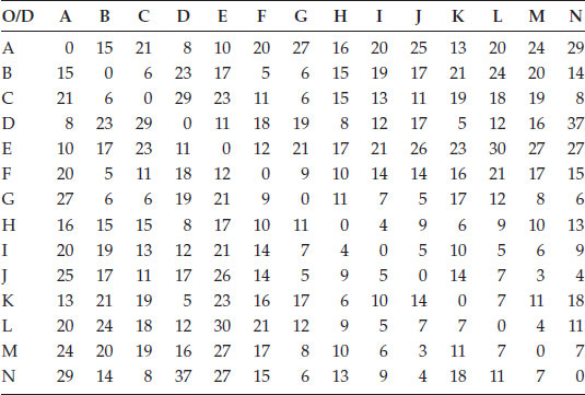
Table 7.1 shows the travel time between any two pairs of cities. This technique is known as origin–destination pairs, and for now we will use it to solve the first version of our problem without the need to use a computer. As you can see, in some instances there is more than one way to move between given origin–destination pairs.

For instance, consider the movement between E and M; you can go through route EFGJM with a duration of 29 minutes, or through route EFIM with a duration of 25 minutes, or through EHIM with a duration of 27 minutes, or through the route EHKLM with a duration of 34 minutes, or through route EHKLIM with a duration of 41 minutes. I will stop here: I could, of course, elaborate more through EABCNJM and many other possible routes.

When solving this type of problem, the decision maker must identify the shortest path between any origin–destination pairs; the shortest path will be defined in terms of the cost, which in this case relates to the travel time.

Final results from all calculations show that node H is the ideal location for the siting of the facility (police station). This conclusion is simply justified because H is the node with the smallest total network travel time of 143 minutes.

TABLE 7.1
Travel Time between Origin–Destination Pairs

A simple summation of travel times per node suffices to reveal the location with the higher degree of accessibility where the police station should be located. In a small case, like the one in the aforementioned example, we can do this by inspection, but in larger problems we need to create a mechanism that explicitly models it.

In a nutshell, we are finding the best routes between origin–destination pairs (OD) and then selecting the location that minimizes the total network travel time. More formally, the identification stage should be the result of solving multiple shortest path sub-problems between all possible combinations of pairs of nodes. Hence, the problem has a combinatorial component, which is not conditioned by the decision variables but rather fixed and linked to its very own geometrical structure. Soon we will tackle a somewhat similar problem of municipal infrastructure in which the problem is also combinatorial but the structure does depend on the decision variables.

The second stage of the facility siting problem is that related to the objective. The problem can be extended when a time restriction is imposed. Consider, for instance, that the maximum travel time from any point must be equal to or less than 15 minutes. This restriction will force us to look for a location where all travel times are smaller than the requested one. In this case, the travel times between H and any other city are smaller than or equal to 15 minutes except between H and A and H and E, where the travel time exceeds by 2 minutes and 1 minute, respectively.

7.3  Shortest Path

The shortest path problem is one of the most recognized optimization algorithms; it is used by travel agents, delivery companies and emergency response vehicles even though you use it whether through for a navigation application to drive or plan your commute trip by public transportation or by booking a flight using any of the available online sites on the Internet. The shortest path problem refers to one in which a traveller wants to find the shortest way to move from a given origin to a given destination. By ‘shortest’ we mean the fastest and, in a general sense, the cheapest. For instance, consider an individual taking the metro to go to work. He or she will find the best way to transfer between metro lines in such a way that minimizes his or her total travel time. Perhaps another user, unfamiliar with the network, may use a rather different definition of ‘shortest’ as that with fewer connections, or a more straightforward way to get there.

The problem could relate to the travel time, distance or the overall cost. For instance, consider a tourist taking a flight for vacation who wants to get to a given destination at the lowest cost; a similar case is that of the driver taking the highways and other fast roads trying to avoid arterial and collector roads because he or she either wants to minimize the likelihood of accidents (cost) or minimize vehicle deterioration by taking roads in better conditions even if that means a slightly longer travel time. Another case is taking some roads with longer travel time that helps avoid paying tolls.

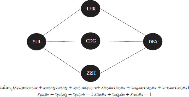
This problem follows a set-up in which each node is given a decision variable (x), which carries the information of origin (i) and destination (j). An enumeration of all possible movements is performed by utilizing those permitted movements at the constraints. The mathematical algorithm for this problem has one objective: to minimize the total cost (c_i,j) and three main constraints, namely, one for the origin, one for the destination and a set of constraints for the network in order to define connectivity. The total cost takes the form of a summation over all possible routes. For this, the connectivity of the network must be defined by enumerating all possible permitted movements in the network.

$\underset{x_{i,j}}{\min }{\displaystyle \sum _{i=1}^N{x}_{i,j}{c}_{i,j}}$

The constraints for the starting and ending nodes depend on the number of travellers; in the classical problem there is one individual. The starting node constraint equates all possible outgoing movements to proximal locations (say indexed by b) directly connected to the starting node (say a) to the number of individuals (one in this case), as shown in the following equation:

${\displaystyle \sum _{b=1}^B{x}_{a,b}=1}$

For simplicity, consider the case depicted in Figure 7.1. Assume that the starting node is A; hence, the first constraint will take the form

$x_{A,D}+x_{A,E}+x_{A,B}=1$

Consider now M as the ending node (Figure 7.1). Assume again that there is one individual travelling. The constraint for such a node will be $x_{J,M}+x_{I,M}+x_{L,M}=1$. In general, the constraint for the ending point (Z) for one individual with nearby arrival nodes indexed by r (as you can see, the total value goes to R, which is just a convention since we do not know how many of them are there) is depicted by the following equation:

${\displaystyle \sum _{r=1}^R{x}_{r,Z}=1}$

Finally, when there are intermediate nodes, we need to define possible in and out movements from such nodes. This type of constraint is the one that really gives structure to the network. All possible movements should be defined. Note: I say possible because for this you need to take into consideration the permitted direction of the travellers’ flow; in most cases, the direction is in both senses, but in some exceptional cases, it may be restricted, or the opposite direction may not make sense at all. For instance, when travelling to another country, it won’t make sense to cross the Atlantic and reach Europe to come back to America and then back again to Europe! Assume we are building this for node c and indexing the arrival nodes by a and destination nodes by d. Then the equation for the intermediate nodes will take the form ‘all in = all out’, as shown as follows:

${\displaystyle \sum _{a=1}^A{x}_{a,c}}={\displaystyle \sum _{d=1}^D{x}_{c,d}}$

It is easier to see this in an example; so let’s look at one concrete case you may be familiar with.

7.3.1  Simple Example of the Shortest Path

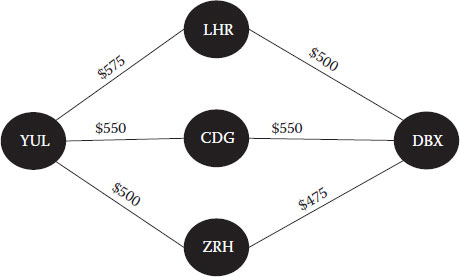
Consider the case of a traveller choosing his or her connections to fly from Montreal (YUL) to Dubai (DBX). Assume the individual prices of flight segments are known, as well as possible connections through London (LHR), Paris (CDG) or Zurich (ZRH). The network of stopovers is given in Figure 7.2, and the complete mathematical formulation is also shown below it.

As you probably realize, I have used airport codes instead of the full airport names. This is because, even without using the actual names, the mathematical formulation turns out to be too long, and hence it is advisable to use just one letter per node to minimize this issue. This letter can represent the actual name or it can be arbitrarily chosen.

The other thing you probably realize is that this problem is somewhat trivial once you know the cost. But don’t jump into a conclusion too fast because defining the cost could be somewhat challenging. You probably remember similar cases in which I combined various criteria into one in the previous chapters. For this case, the cost could comprise the actual monetary cost combined with flight comfort (first, business or economy seat?), the total travel time and whether the flights are overnight or not (to help you adjust to jet-lag), stopover convenience (perhaps you prefer a flight stopping for hours to be able to see a new city!), arrival and departure time (some people may not care for this) or whether you make air miles (very important to me, I actually use this as an initial filter).

Let’s say I weighed all these criteria, as shown in a previous chapter, and the final cost is given in Figure 7.3. Hence, it is simple to see that the solution involves only two nodes with values of 1, x_yul,zrh = 1, x_zrh,dbx = 1, and all others with values 0, x_yul,lhr = 0, x_yul,cdg = 0, x_cdg,dbx = 0, x_lhr,dbx = 0. The objective value would be 975.

FIGURE 7.2
One-scale flight network.

FIGURE 7.3
One-scale flight network with costs.

7.3.2  Extended Example of the Shortest Path

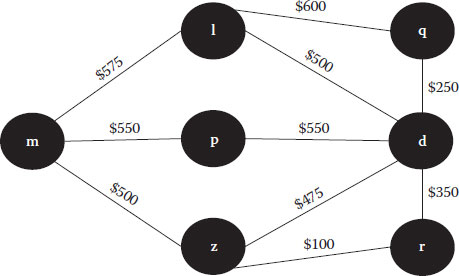
Let’s now extend the example. Consider you just have discovered that there are other routes with more stops (two each) in addition to the previous routes. Figure 7.4 illustrates this expanded network used in this section.

FIGURE 7.4
An expanded flight network.

The first thing we will do is change the airport codes to single letters; so Montreal (m), London (l), Paris (p), Zurich (z), Qatar (q), Dubai (d) and Rome (r) would be our possible choices.

In this formulation, we need to make use of constraints for the starting and ending nodes as well as for the intermediate nodes (l and z when connecting to q and r).

So far, this problem looks like the previous one; so to make it more interesting, let us say there are two travellers (you and your friend). The nodes that take values would need to take a value of either 2 or 0 because you want to be in the same plane as your very dear friend (won’t you?). This will require the inclusion of additional constraints stipulating that the nodes take the values 0 or 2. In the case of various unrelated travellers, we do not need to impose such a constraint.

The objective takes the same form; the only difference is that there are more nodes, and the cost for the new possible movements needs to be defined a priori (in advance). The constraints also take the well-known form; the departure node constraint is the same (except that the number of travellers is equal to two). The arrival constraint has more possibilities by adding the combinations Qatar (q) and Rome (r).

$\begin{array}{l}\underset{x_{i,j}}{\min }(x_{m,l}{c}_{m,l}+x_{m,p}{c}_{m,p}+x_{m,z}{c}_{m,z}+x_{l,d}{c}_{l,d}+x_{p,d}{c}_{p,d}+x_{z,d}{c}_{z,d}+x_{l,q}{c}_{l,q}\hfill \\ \begin{array}{l}+x_{z,r}{c}_{z,r}+x_{r,d}+x_{q,d}{c}_{q,d})\\ x_{m,l}+x_{m,p}+x_{m,z}=2\end{array}\hfill \\ x_{l,d}+x_{p,d}+x_{z,d}+x_{q,d}+x_{r,d}=2\hfill \\ x_{i,j}=(0,2)\forall i,j\hfill \end{array}$

We also need to define the intermediate node constraints; they will take the following form: x_m,l = x_l,d + x_l,q and x_m,z = x_z,d + x_z,r. Note we have not used the possible connections between London and Paris and Paris and Zurich. I will leave this to you as home practice. Simply add an expression for the cost and proceed in the same manner as before.

One thing that probably crossed your mind is why we have to write down all combinations at the objective even though some would not be used. The answer lies in the fact that you want to define all possibilities first, and then you choose the most convenient one (typically the cheapest); the circumstances that define the most convenient one may change along the way, and then you may find yourself revisiting the problem. So if the structure is in place, you can deal with any changes and will be able to make decisions even under changing circumstances.

This is typical of optimization problems, where we run scenarios to answer specific questions and examine alternative solutions. We will see a more detailed case of scenarios in the following chapter, but it is applicable anywhere. If you change from one decision maker to another, the new individual’s definition and weighing of the cost will likely be different from those of the first one.

The shortest path is used in many applications in real life: websites of travel agencies and airlines, navigation systems, public transportation applications, etc.

7.4  Transportation (Distribution or Allocation)

The transportation problem is nothing but the identification of supply and demand forces from origins (O) to destinations (D). The purpose is to identify the amounts that will go between OD pairs. Think of a company that manufactures the same product at several factories across Asia and ships the goods out of seaports to locations where they are demanded. Picture, for instance, computers produced in Hong Kong, Singapore and Shanghai heading to Los Angeles, New York and Panama. How the computer goes from the factory to the port is itself another problem, which we will address soon. The transportation problem does not worry about roads or routes but rather concentrates on finding the cheapest way to move the goods from the origin to the destination. The fact that a factory is more competitive and can afford to sell at the lowest prices is central to this problem; goods out of that factory will be moved first. But eventually it will run out of commodities, and the second cheapest should provide goods until it reaches its capacity, then the third one, and so on. To make it simple, the supply and demand will be assumed to be at equilibrium, that is, the number of goods supplied matches with the demand. Then this assumption will be relaxed and the supply will be much larger than the demand. Demand in that event will be known.

Costs are associated with origin–destination pairs, which assumes that in each pair the cheapest route had been identified. How the route goes is not relevant in the scope of this problem; it all comes down to a final cost per route.

The solution takes the form of the number of units shipped between the origin and the destination, that is, how many units are moved from Hong Kong to New York, from Hong Kong to Los Angeles, from Hong Kong to Panama, then from Singapore to each of the three destinations, and from Rotterdam to each of them again. At the end, for this case you have nine possible combinations of origin–destination pairs, along with the number of units moved between them.

The algorithm behind this type of problem takes the form of one objective and two major constraints. The objective is the common minimization of the total cost, with the decision variable being the number (x) moved from the origin (i) to the destination (j). The total cost is found by multiplying individual cost (c_i,j) with the corresponding amounts (x_i,j).

$\underset{x_{i,j}}{\min }{\displaystyle \sum _{i=1}^N{x}_{i,j}{c}_{i,j}}$

The first constraint deals with the equilibrium of the numbers exported out of a given origin: it makes the summation of all goods out of that origin to any possible destination (D_i) equal to the total available supply at such origin. The second constraint does the same but for a given destination, that is, it sums across origins (O_i) to a common destination.

$\begin{array}{ll}{\displaystyle \sum _{j=1}^N{x}_{i,j}=O_i,}\hfill & \text{for }i=1,2,\mathrm{3\dots }\hfill \\ {\displaystyle \sum _{i=1}^N{x}_{i,j}=D_j,}\hfill & \text{for }j=1,2,\mathrm{3\dots }\hfill \end{array}$

Lack of equilibrium results in a slight modification on the previous equations: goods available at a given origin (Oi for a given i) may not have been totally utilized, hence the ‘smaller than’ inequality. This is certainly true when goods are more expensive and hence left to completely unsatisfied demand at a given destination. The equation for demand remains an equality if we enforce the assumption that demand will be satisfied; on the contrary, the equality will turn out to be a ‘bigger than’ inequality if the demand (Dj for a given j) is not satisfied or suppliers send more goods than possibly required to a given destination (remember containers will force you to round up your number of shipped units, and demand is difficult to estimate, so you may actually ship more units at the end of the day).

$\begin{array}{ll}{\displaystyle \sum _{j=1}^N{x}_{i,j}\le O_i,}\hfill & \text{for }i=1,2,\mathrm{3\dots }\hfill \\ {\displaystyle \sum _{i=1}^N{x}_{i,j}\ge D_j,}\hfill & \text{for }j=1,2,\mathrm{3\dots }\hfill \end{array}$

In addition to the previous constrains, the number of goods needs to be positive (x_i,j ≥ 0) depending on the type of goods being moved, and it could be restricted to be integers (x_i,j ∈ Z), strictly speaking for all pairs of i, j.

7.4.1  Simple Example of Transportation

Let’s take the case of mobile phones produced in Hong Kong (k), Shanghai (s) and Beijing (b) and shipped to the United States for sale in New York (n), Houston (h) and Los Angeles (l). You can think of them as coming from the same company (whichever you prefer). The objective is to minimize the total cost:

$\underset{x_{i,j}}{\min }{\displaystyle \sum _{i=1}^N{x}_{i,j}{c}_{i,j}}$

In this case, we can explicitly write it for the given nodes, so it takes the form

$\begin{array}{l}\underset{x_{i,j}}{\min }{x}_{k,n}{c}_{k,n}+x_{k,h}{c}_{k,h}+x_{k,l}{c}_{k,l}+x_{s,n}{c}_{s,n}+x_{s,h}{c}_{s,h}+x_{s,l}{c}_{s,l}+x_{b,n}{c}_{b,n}\\ +x_{b,h}{c}_{b,h}+x_{b,l}{c}_{b,l}\end{array}$

For this case, we have six constraints for the origins (supply–manufactures) and six additional constraints for the destinations (demand–locations). Assume that the corresponding capital letters for each city represent the number being produced or demanded at each one of them; that is, K, S and B represent the production out of Hong Kong, Shanghai and Beijing, respectively. For New York, Houston and Los Angeles, we will use N, H and L to represent the numbers being demanded. For instance, x_k,n means the number produced at k being used to satisfy the demand at n. Once again, the inequality is smaller or equal, given the fact that not necessarily all production will sell.

$\begin{array}{l}{x}_{k,n}+x_{k,h}+x_{k,l}\le K\\ x_{s,n}+x_{s,h}+x_{s,l}\le S\\ x_{b,n}+x_{b,h}+x_{b,l}\le B\end{array}$

For the destinations, the constraints look much like those of the origins, except in the sense of the inequality. As expected, the inequality is greater or equal, given the fact that the demand is an estimation and you don’t want to fall short of supplying at least as much as required and perhaps some extra units, just in case.

$\begin{array}{l}{x}_{k,n}+x_{s,n}+x_{b,n}\ge N\\ x_{k,h}+x_{s,h}+x_{b,h}\ge H\\ x_{k,l}+x_{s,l}+x_{b,l}\ge L\end{array}$

Again, just as in the case of the shortest path, we arrive at the point at which the cost is key to the solution. Once again, the cost in this case relates to many elements, such as the carrier’s fees and the total travel time. The solution will identify the number of goods from given sources to supply to the destinations, but will not be concerned with the selected route. Route selection leads again to the shortest path problem.

Let’s assume that the costs (Table 7.2) are provided to you by the analyst who has compared air transportation versus sea transportation and many possible routes and carriers and who finally identified the most convenient route for each pair (origin–destination).

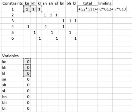
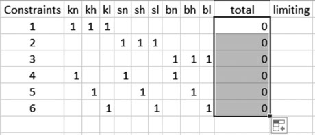
We will illustrate the use of Excel in Figure 7.5. First, the problem needs to be defined in such a way that the structure is represented explicitly and all elements whose value may change are defined in terms of the other elements with fixed or constant values. Let’s see; first, let’s place on a spreadsheet the coefficients next to each variable in order to define the constraints. Enumeration of pairs of origin–destination is defined: kn, kh, kl, sn, sh, sl, bn, bh, bl. Then, they are also defined as variables in another region of the spreadsheet. To define the first constraint, we multiply each coefficient by the variable, so, for instance, the first constraint only has coefficients of 1 for those elements present at it (kn, kh, kl); the rest carry a zero next to them (sn, sh, sl, bn, bh, bl).

The multiplication continues for all remaining coefficients with the corresponding variables. This exhaustive multiplication facilitates the definition of all remaining constraints by simply copying it to the other ones as shown in Figure 7.6.

TABLE 7.2
Origin–Destination Costs

Origin/Destination	New York (n)	Houston (h)	Los Angeles (l)
Hong Kong (k)	1400	1200	900
Shanghai (s)	1300	1100	800
Beijing (b)	1200	1500	1000

FIGURE 7.5
Problem definition.

FIGURE 7.6
Constraint set-up.

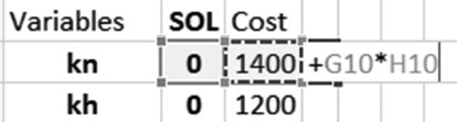
Next, we need to define the objective. For this purpose, we add the cost of each pair and multiply the binary decision variable by the cost, as shown in Figure 7.7.

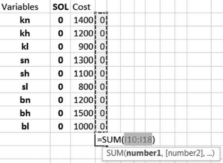
The objective is the overall summation of the cost for all links, as shown in Figure 7.8. For those selected, the decision variable will take the number of units assigned; for the others it will be zero.

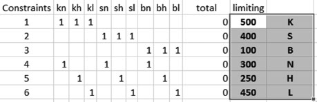
The next step is to bring the limiting values next to each constraint, as shown in Figure 7.9, and invoke the solver tool located at the DATA tab of Excel.

FIGURE 7.7
Objective set-up for one variable.

FIGURE 7.8
Objective set-up across variables.

FIGURE 7.9
Limiting values on the constraints.

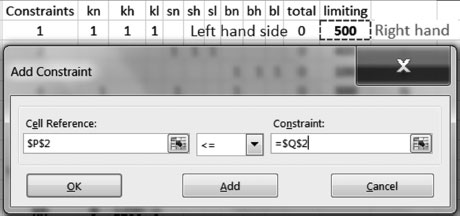
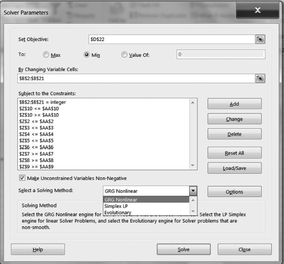
We invoke the solver and select the objective cell (with the summation of cost) and the constraints. The constraints require the definition of the left-hand side and the right-hand side, as shown in Figure 7.10.

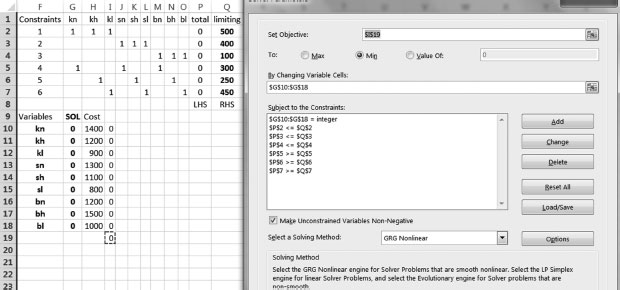
All other constraints should also be defined. After that, one needs to specify the decision variables. The final problem set-up on Excel is shown in Figure 7.11.

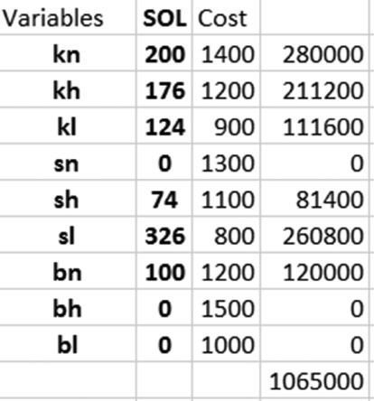
The final solution is then identified by clicking on solve. This populates the cells corresponding to the decision variables with the optimal values, as shown in Figure 7.12.

FIGURE 7.10
Solver: definition of the left-hand side.

FIGURE 7.11
Final problem set-up in Excel.

FIGURE 7.12
Optimal values for the decision variables.

7.5  Trans-Shipment

The trans-shipment problem looks much like the shortest path, but it is really an extended version of it. Trans-shipment allows flows of commodities coming into some nodes: you can think of them as the location of airports, ports, or simply entry points, that is, locations where flows from outside the system come into it. Flows exiting the network are also permitted. We typically use arrows pointing outwards to represent exiting movements and arrows pointing inwards to denote income flows. In trans-shipment, we could find several links being used to move goods.

The constraints for this type of problem follows one general rule already used in the shortest path: all incoming flows equal all outgoing flows. However, among incoming flows one can have interior (x_i,j) and exterior flows coming in (I), and among outgoing flows they can head towards an interior (x_i,j) or exterior location (E). The following is the generic constraint used for this type of problem; soon we will see its application in a couple of true examples. Interior flows coming in are indexed by i, whereas those heading out but into interior nodes are indexed by j.

${\displaystyle \sum _{i=1}^N{x}_{i,j}}+I={\displaystyle \sum _{j=1}^M{x}_{i,j}+E}$

The objective is just a replica of the shortest path objective and the transshipment objective, that is, to minimize total cost given by a multiplication of unitary cost by the number of units on the link, which is shown here:

$\underset{x_{i,j}}{\min }{\displaystyle \sum _{i=1}^n{\displaystyle \sum _{j=1}^m{x}_{i,j}{c}_{i,j}}}$

7.5.1  Example of Trans-Shipment for Canadian Airports and Roads

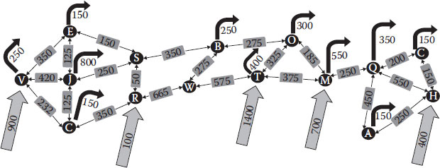
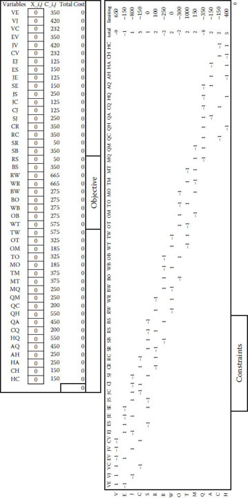
This example illustrates an application of the trans-shipment algorithm (Figure 7.13). Assume you have international passengers arriving at Canadian airports in Vancouver (V), Regina (R), Toronto (T), Montreal (M) and Halifax (H). Passengers rent cars and head to their favourite destinations; for simplicity we will exclude those passengers taking local flights and assume that all individuals in our network have chosen to move by highways. The highway network is shown in Figure 7.13; the numbers over the arrows represent cost (in this case distance in kilometres), the grey arrows are the flows of international passengers in hundreds of thousands, and the black arrows represent outgoing flows exiting the system at specific cities. The codes for cities are Vancouver (V), Calgary (C), Jasper (J), Edmonton (E), Regina (R), Saskatoon (S), Winnipeg (W), Thunder Bay (B), Toronto (T), Ottawa (O), Montreal (M), Quebec (Q), Saint Andrews (A), Charlottetown (C) and Halifax (H).

The set-up of constraints is given in Table 7.3; it is convenient as you will learn after this chapter to write the constraints before coding your software (Excel in this case). For the trans-shipment problem, we require one constraint per node, so in total we will have 15 constraints as follows. For the formulation on Excel, we need to move all variables to one side and amounts to the other side; I have chosen to move all variables to the left-hand side and amounts to the right-hand side. As you can see in Figure 7.14, we are looking at 46 origin–destination pairs.

FIGURE 7.13
Canadian network.

TABLE 7.3
Definition of Constraints for Canadian Network

Node	Constraint
V	$900+x_{E,V}+x_{J,V}+x_{C,V}=250+x_{V,E}+x_{V,J}+x_{V,C}$
E	$x_{V,E}+x_{J,E}+x_{S,E}=150+x_{E,V}+x_{E,J}+x_{E,S}$
J	$x_{V,J}+x_{E,J}+x_{C,J}+x_{S,J}=800+x_{J,V}+x_{J,E}+x_{J,C}+x_{J,S}$
C	$x_{V,C}+x_{J,C}+x_{R,C}=150+x_{C,V}+x_{C,J}+x_{C,R}$
S	$x_{E,S}+x_{J,S}+x_{R,S}+x_{B,S}=x_{S,E}+x_{S,J}+x_{S,R}+x_{S,B}$
R	$100+x_{C,R}+x_{S,R}+x_{W,R}=x_{R,C}+x_{R,S}+x_{R,W}$
B	$x_{S,B}+x_{W,B}+x_{O,B}=250+x_{B,S}+x_{B,W}+x_{B,O}$
W	$x_{R,W}+x_{B,W}+x_{T,W}=x_{W,R}+x_{W,B}+x_{W,T}$
O	$X_{B,O}+x_{T,O}+x_{M,O}=300+X_{O,B}+x_{O,T}+x_{O,M}$
T	$1400+x_{W,T}+x_{O,T}+x_{M,T}=400+x_{T,W}+x_{T,O}+x_{T,M}$
M	$700+x_{T,M}+x_{O,M}+x_{Q,M}=550+x_{M,T}+x_{M,O}+x_{M,Q}$
Q	$x_{M,Q}+x_{A,Q}+x_{C,Q}+x_{H,Q}=350+x_{Q,M}+x_{Q,C}+x_{Q,H}+x_{Q,A}$
A	$x_{Q,A}+x_{H,A}=150+x_{A,Q}+x_{A,H}$
C	$x_{Q,C}+x_{H,C}=150+x_{C,Q}+x_{C,H}$
H	$400+x_{Q,H}+x_{C,H}+x_{A,H}=x_{H,Q}+x_{H,C}+x_{H,A}$

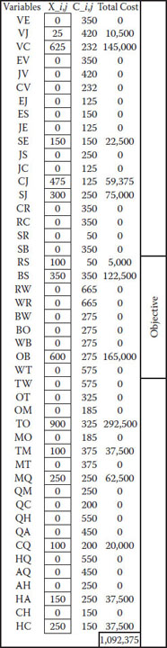
Figure 7.15 shows the solution for the network: from Vancouver, 25 travellers will go to Jasper and 625 to Calgary, from Saskatoon to Edmonton 150, from Calgary to Jasper 475, from Regina to Saskatoon 100, Thunder Bay and Saskatoon 350, Ottawa and Thunder Bay 600, Toronto and Ottawa 900, Toronto and Montreal 100, Montreal and Quebec 250, Charlottetown and Quebec 100, Halifax and Saint Andrews 150 and Halifax and Charlottetown 250. The rest of the nodes receive no travellers.

7.6  Allocation of Public Works

The optimization of allocations is nothing but an application of the transportation (distribution) problem in the world of public affairs, to be precise in the tendering process for public infrastructure construction or maintenance. Think of a municipality or any agency trying to allocate public works among contractors. In the language of the transportation problem, each contractor will represent a source and each region in town a destination. The most common way to look at this problem is when a country wants to award public infrastructure maintenance contracts for the coming year. Regions in a country or town are typically chosen to match corridors of interest or zones that are geographically separated from others.

FIGURE 7.14
Objective and constraints for Canadian network.

FIGURE 7.15
Solution for Canadian network.

The objective is to minimize total cost, but let me stop you right there. Cost in this case, as in many others, is not only the plain monetary figure that the bidder wrote in his or her bid: no! it should comprise other elements such as the bidder technical capability to undertake the task, and perhaps also their history of previous works (experience) and their financial capability. In some tendering processes, this is separated as a first stage in which an initial filter based on financial and technical capabilities is inserted to reduce the number of bidders so that in the second stage only those that had met with the aforementioned criteria are considered. For the rest of this section, we will assume you have already incorporated the experience together with the cost. Here are two ideas of how you can do this: through a weighted expression, in which you can (a) monetize experience and subtract it from cost or (b) bring both elements to a non-monetized base, by considering the likelihood of successful achievement of the project in a 0–10 scale and then adding to it the number of similar scale projects up to 10.

For us, the capability will be explicitly considered in the formulation, and the use of an initial filter can rule out risky/inexperienced tenders. Let’s get the formulation: consider a municipality tendering public works contracts containing packages of roads, sewage and water-main maintenance and repairs (this would be prepared by a coordination approach, which I will explain in the next section). The sources are the contractors with limited construction capability (amount of goods), and the destinations are the urban zones or regions within a municipality in which annual construction works (for infrastructure) need to be done and awarded (allocated) to a contractor. The objective is to distribute the construction projects for all areas to the lowest bidders. Assume we have m contractors in total, indexed by i, and n regions, indexed by j. The contractor’s maximum construction capacity is given by a_i and the total amount of work required at a given region by b_j. In this problem, c_i,j denotes the unitary cost of construction, which could be for maintenance, rehabilitation or upgrading per metre of pipe or square meter of road. This cost is unique for a given contractor i on a given region j. Finally, let y_i,j denote the total amount of work awarded to contractor i on region j, which is not necessarily equal to his or her capacity (a_i). In this context, the problem takes the following objective:

$\underset{y_{i,j}}{\min }{\displaystyle \sum _{i=1}^n{\displaystyle \sum _{j=1}^m{y}_{i,j}{c}_{i,j}}}$

This will be subject to two constraints. The first one is for the contractor’s capacity, which cannot be exceeded:

${\displaystyle \sum _{i=1}^m{y}_{i,j}\le a_i}$

The other constraint is for the amounts required at a given region (or zone). The total amount of work allocated to contractors in region j cannot exceed the total amount of work b_j required in that zone.

${\displaystyle \sum _{j=1}^n{y}_{i,j}\ge b_i}$

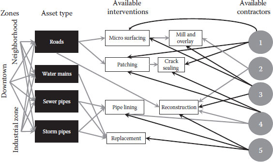
This problem can be formulated in a reverse way, that is, considering contractors to be destinations and regions/zones to be sources. Disregarding the approach, the mechanism is a simple matching process in which we identify the amounts allocated to origin–destination pairs. Figure 7.16 illustrates such a concept for five contractors, three regions and four types of interventions. As seen, interventions in different zones of the town are allocated based on each contractor’s area of expertise and the quoted cost.

Depending on their location, some contractors will be cheaper than others. One mainstream belief is that local contractors would have less expensive bids compared to those based at far locations (external), mostly because they have temporary relocation cost added to their overall cost structure when bidding for a project. However, other elements such as technology (machine productivity) may make some contractors (even if not locals) more competitive above certain levels of scale (amount of works). Hence, putting together a good package per zone and awarding it in such a way is sometimes preferable to tendering individual repairs per road segment. Section 7.7 explains the basics on how to identify which public works to bundle together by employing a coordination of works approach. The following section contains an example that hopefully will illustrate the applicability of awarding public works.

FIGURE 7.16
Allocation of works to contractors.

7.6.1  Example of Public Works Awarding

Consider the case of five contractors: let’s assume we are talking about one job only, namely, pipe replacement, and that the cost shown in Table 7.4 is the unitary cost per linear meter. The regions are downtown (d), highway frontage (h), industrial park (p) and Rosedale residential (r) (Table 7.1).

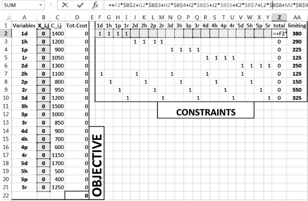
The rest of the problem concentrates on identifying the amounts allocated to contractor–region pairs. It is useful, however, to explicitly write the constraints before we transfer them into an Excel spreadsheet; let’s see for contractors whether we may fully utilize their capability a_i or not. Let’s assume the contractors’ total capabilities are 1 = 380, 2 = 290, 4 = 225, 3 = 125, 5 = 150.

$\begin{array}{l}{x}_{1,d}+x_{1,h}+x_{1,p}+x_{1,r}\le a_1=380\\ x_{2,d}+x_{2,h}+x_{2,p}+x_{2,r}\le a_2=290\\ x_{3,d}+x_{3,h}+x_{3,p}+x_{3,r}\le a_3=225\\ x_{4,d}+x_{4,h}+x_{4,p}+x_{4,r}\le a_4=125\\ x_{5,d}+x_{5,h}+x_{5,p}+x_{5,r}\le a_5=250\end{array}$

TABLE 7.4
Contractors and Their Capabilities

Contractor/Region	d	h	p	r
1	1400	1200	900	1050
2	1300	1100	800	950
3	1200	1500	1000	850
4	900	700	600	1150
5	1700	500	400	1250

For regions, we want to make sure that we allocate all the works that are required this year (bj); this is, of course, an estimation of works, and along the way, there may be changes mostly in the direction of increasing needs with additional areas to be paved/repaired (remember, though you observe the condition and make the planning, it takes 1 year before you actually do the construction work, so things may have gotten a bit worse). Let’s assume the municipality has a budget of $1 M for this work and that the following amounts of work are being demanded per region: d = 125, h = 150, p = 550, r = 325.

$\begin{array}{l}{x}_{1,d}+x_{2,d}+x_{3,d}+x_{4,d}+x_{5,d}\ge b_d=125\\ x_{1,h}+x_{2,h}+x_{3,h}+x_{4,h}+x_{5,h}\ge b_h=150\\ x_{1,p}+x_{2,p}+x_{3,p}+x_{4,p}+x_{5,p}\ge b_p=550\\ x_{1,r}+x_{2,r}+x_{3,r}+x_{4,r}+x_{5,r}\ge b_r=325\end{array}$

Figure 7.17 shows the final set-up in Excel. As you can see, I have transferred the constraints directly into the right box and the objective into the left box. Also, remember that each constraint is the product of a coefficient on the constraint table and the value of X_i,j. As you can notice, the definition of constraints follows the same order of the constraint equations previously shown.

FIGURE 7.17
Excel set-up for contractor allocation.

FIGURE 7.18
Solver set-up for contractor allocation.

The set-up in the solver window is shown in Figure 7.18. As you can see, all constraints are given in rounded units (integers); the objective corresponds to the cell that minimizes total cost, and the decision variables match the cells that we need to estimate.

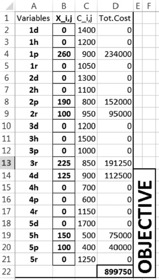
The final solution is shown in Figure 7.19. As can be seen, the industrial park works will be allocated to three contractors (1, 2 and 5), the works on Rosedale residential subdivision to two contractors (2 and 3), the works on downtown exclusively to contractor 4 and the works to highway frontage to one contractor (5).

The problem can be generalized to a more real setting. Consider the case of many types of interventions: say, pipe lining and pipe replacement along with road reconstruction and crack sealing, just to name a few. It could be the case that contractor’s expertise is unique to one type of infrastructure, but some large contractors do have expertise across the board of public infrastructure assets. I will leave the formulation of this problem as an home exercise; however, as hints, consider that you need to create one spreadsheet per intervention. So in the case, we just spell out, and you will need four spreadsheets.

FIGURE 7.19
Final solution for a contractor allocation.

7.7  Coordination of Public Works

Results from long-term planning of civil infrastructure maintenance and rehabilitation (explained in the following chapter) include the optimal schedule of what physical assets to fix and when to fix them on an annual basis. However, raw results from any long-term analysis produce actions randomly scattered across space and time that do not reflect any measures of coordination or operational efficiency, potentially producing many small contracts that would translate into constant disruption of services to the users (public at large) and higher cost to the government (more bids, inspections, relocation of machinery, transporting materials, etc.). Also, uncoordinated actions between different systems (roads and pipes, for instance) may result in utility cuts in the form of premature damage to recently rehabilitated assets (pavements). Therefore, it’s in the best interest of departments of transportation and municipalities to prepare medium-range tactical plans that are able to advance or defer interventions across different types of adjacent infrastructure, achieving minimal service disruptions and closure of roads, yet staying close enough to optimal results from the strategic analysis.

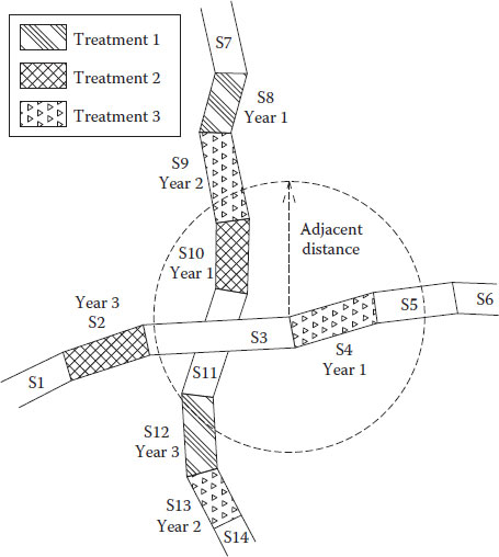
In this section, we will learn the basics of space/time coordination applied to civil infrastructure. The coordination of activities is achieved by clustering together some nearby assets that received treatments within a given time window (but not all). When conducting coordination, we need to consider segments within a specific distance (adjacent distance) with interventions scheduled within a given range of time (temporal distance). Temporal distance is the periods of time that an intervention can be deferred or advanced from its original scheduling. These two constraints identify those segments of infrastructure that are candidates and will be possibly cluster together. For example, as illustrated in Figure 7.20, within the prescribed adjacent distance, segments 4 and 10 are receiving treatments 2 and 3, respectively, in year 1, while segment 9 is receiving treatment 3 in year 2, and segment 12 is receiving treatment 1 in year 3. Assuming that the temporal distance is set to 2 years, these four segments will be grouped together, creating a new group of asset segments (group 1).

FIGURE 7.20
Coordination of works.

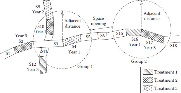
FIGURE 7.21
Coordination: Time and space openings.

Figure 7.21 illustrates the concepts of time and space openings. Recalling from the previous example, segments 4, 9, 10 and 12 were assigned into group 1; similarly, group 2 could have been formed by joining segments 16 and 17. These two groups can now be joined if they are within a distance called ‘space opening’, which indicates the willingness of accepting separation between two groups scheduled on the same year if by operational standards it makes more sense to assign them to the same contractor or undertake both projects (groups) at the same time. An extension to this concept is that of ‘time opening’ in which two groups placed spatially within an acceptable space opening but separated in time (scheduled at different periods) can be joined for similar reasons as noted earlier. This results in a second temporal movement (advance or deferral) of the assets in one of the groups to match the other.

Other elements must be taken into account for performing an analysis capable of developing coordinated tactical plans. Besides spatial and temporal constraints, one must consider the compatibility of actions for the generation of groups (called ‘blocks’ by the software). Not all maintenance and rehabilitation actions can be implemented together. This consideration depends on the agency’s decision, resources, contractor’s specialization, compatibility of machinery, time required per task, etc.

7.7.1  Simple Example of Coordination

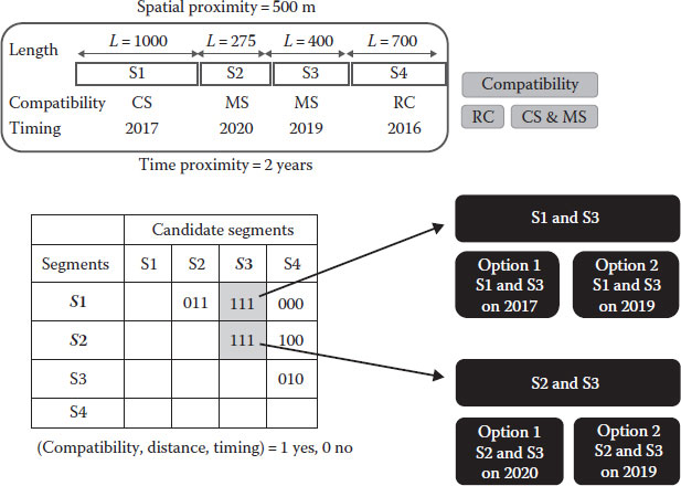
Let’s look at the case of four segments of a road corridor (S1, S2, S3 and S4) receiving various types of maintenance and rehabilitation interventions (Figure 7.22). We will use a binary indicator (0,1) for each criterion, and only pairs of segments with all three criteria (1,1,1) will be chosen as candidates to be scheduled together.

FIGURE 7.22
Coordination set-up.

The first step is to apply a filter of compatibility for the interventions. Assume CS and MS are compatible; this initial filter gives a value of zero to segment S4 (receiving RC). Then we look at 500 m adjacency and identify that for segment S1 both S2 and S3 are within such distance. The space criteria will potentially enable us to pack all three segments together. However, we still need to look at time proximity, set to be 2 years in this example. This rules out the possibility of having S1 and S2 together because their timing is separated by 3 years.

The solution to a coordination problem is a set of clustered segments, which satisfy all three criteria (compatibility, distance and timing). When two segments are packed together, you end up with two possible timings for the actual completion of works. Looking at the case of S1 and S3, one can either advance S3 from 2019 to 2017 or defer the timing for S1 from 2017 to 2019, so there are two possible timings. In this case of three segments packed together (not illustrated in the example), there could be up to three options for timing. Selection of the best timing requires another optimization similar to that presented in the following chapter.

7.8  Network Flows

Consider the case of a network of roads and the need for planners to estimate the demand (number of vehicles) at each link of the network. This problem can be partially solved if we count vehicles at each link of the network; however, this is a daunting task. Even if we know the number of vehicles at given points, still sometimes we may be interested in knowing where the trip originated and where it ended. The same is true for different times of the day and the purpose of the trip; however, I won’t go into this level of detail.

It is likely that you have some information about the entry and exit points and that you may have some counts at mid-segment points (i.e., segments without entries or exits). Let’s call x_i,j the flow of traffic entering at i and exiting at j. The summation over all destinations for the flow entering at i must be equal to the entry rate at i. In other words, all vehicles that entered at a specific point ramp to a highway (i) must exit somewhere, so when you add them all up, they should add to that number.

${\displaystyle \sum _{j=i+1}^n{x}_{i,j}=a_i}$

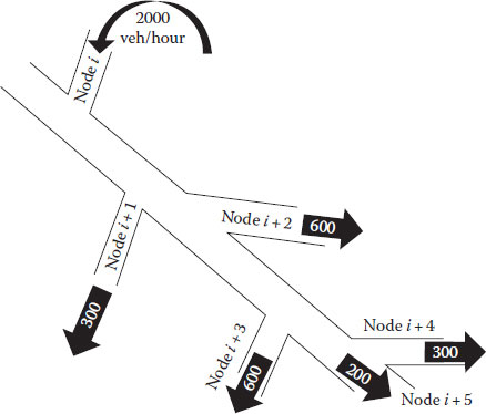
Figure 7.23 illustrates such an example with concrete numbers of a specific case. The entry rate of 2000 vehicles per hour at node i will exit the system at different nodes: 300 at i + 1, 600 at i + 2, etc.

The same is true for all vehicles exiting at a given point (say j); they entered the system somewhere (between 1 and j − 1).

${\displaystyle \sum _{i=1}^{j-1}{x}_{i,j}=b_i}$

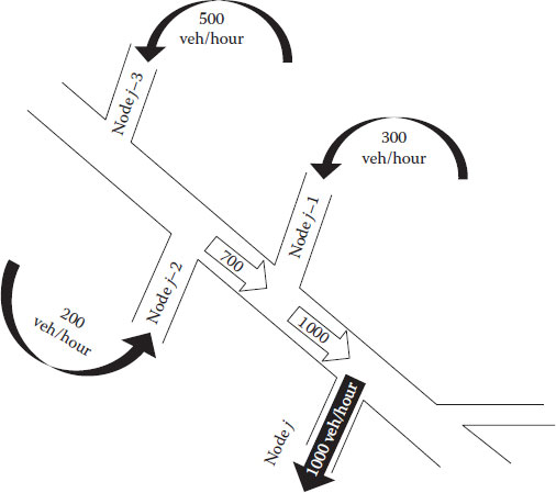
Following the previous example, Figure 7.24 illustrates the case of 1000 vehicles per hour (exit rate) at node j that entered the system at different nodes: 500 at j − 3, 200 at j − 2 and 300 at j − 1.

The objective of this type of problem is to minimize the (square of the) differences between the observed and predicted flows. Assume for now you only have one control point located between the nodes i and i + 1. The summation of all entering flows from 1 to i heading to nodes after i + 1 minus the observed flow between i and i + 1 must be minimized:

$\min \left({\displaystyle \sum _{i=1}^i{\displaystyle \sum _{i=i+1}^n{x}_{i,j}}}\right)-q_{i,i+1}$

FIGURE 7.23
Example of a vehicle flow.

FIGURE 7.24
Vehicle flow in a road network.

In the example presented in Figure 7.24, we have seven nodes; the known flow rate is located between nodes 3 and 4. Hence, the double summation can take on origin the values between 1 and 3 and the destination values between 4 and 7. Let’s explicitly state the double summation:

$x_{1,4}+x_{1,5}+x_{1,6}+x_{1,7}+x_{2,4}+x_{2,5}+x_{2,6}+x_{2,7}+x_{3,4}+x_{3,5}+x_{3,6}+x_{3,7}$

The observed flow is called q_3,4, and therefore the objective can be stated as follows:

$\begin{array}{l}\min (x_{1,4}+x_{1,5}+x_{1,6}+x_{1,7}+x_{2,4}+x_{2,5}+x_{2,6}+x_{2,7}+x_{3,4}\\ +x_{3,5}+x_{3,6}+x_{3,7})-q_{i,i+1}\end{array}$

The desired value of the objective is zero; for this, we can use the Excel solver, and instead of using a minimization, we could set the target value of the objective to be zero.

7.8.1  Example: Pedestrians’ Tunnel Network

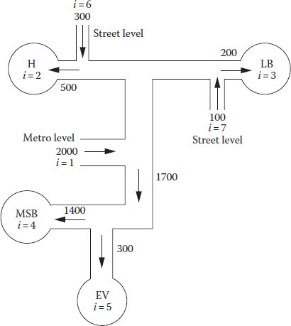
Let’s solve an example of the system of tunnels at Concordia University in Montreal. Figure 7.25 presents a simplified version of it; buildings are represented by circles, and notice that the indexing of nodes is arbitrarily done.

The objective is to minimize the summation of flows between 2, 6, 3, 7 and 1 exiting at 4 or 5, minus the actual flow observed at the segment after 1 and before 4 (q_1,4) of 1700 pedestrians per hour. However, nodes 2 and 3 are terminal nodes (imagine all students are heading to class at such buildings).

$\min \left(x_{6,4}+x_{6,5}+x_{7,4}+x_{7,5}+x_{1,4}+x_{1,5}\right)-\left(q_{1,4}=1700\right)$

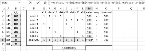
The objective is that the summation of predicted flows (x_6,4 + x_6,5 + x_7,4 + x_7,5 + x_1,4 + x_1,5) must equal to the observed flow in the segment located between 1 and 4, which is represented at the bottom of the constraints’ box. The other constraints can be easily read from Figure 7.26.

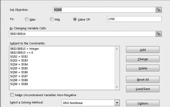
Figure 7.27 shows the set-up of solver add-in on Excel. Notice that the objective is not a maximization or a minimization; rather, it is to find a specific value for the summation of predicted flows. In this case, the target value is 1700. The decision variables are selected as the range from B2 to B14, the type of decision variables is specified to be integers and positive, and then the other constraints are coded as you can see on the interface shown in Figure 7.27.

FIGURE 7.25
Pedestrians at underground tunnels.

FIGURE 7.26
Excel set-up for underground tunnels.

FIGURE 7.27
Solver set-up for underground tunnels.

Exercises

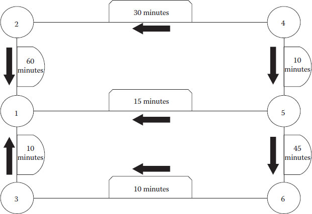
1.  A traveller is trying to go from node 4 to node 1 (Figure 7.28). Formulate and solve the shortest path problem using travel time as cost.

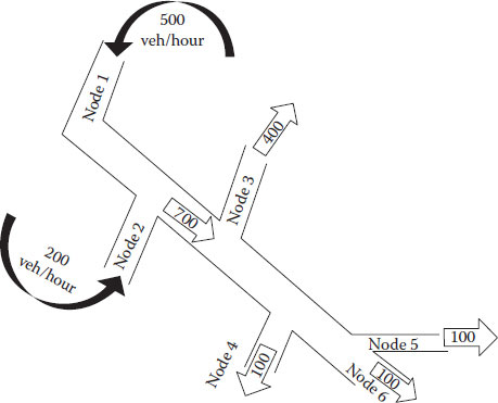
2.  Prisoners are planning to escape from jail in a dictatorial country. Help them plan the escape route: identify number of prisoners per link and the overall route to follow (use a trans-shipment formulation). Figure 7.29 shows the network of escape tunnels (one direction of movement). Travellers start at nodes 4 (12 travellers), node 5 (6 travellers) and node 6 (13 travellers). All travellers are going to node 1 (liberty!). Travel time for every link along with a sense of strictly permitted movement is shown over every link. Formulate the problem.

3.  Modify the formulation of Exercise 7.1 and reverse the direction of arrows; the departure point now is node 1 and the arrival point is node 4.

4.  Modify the formulation of the objective by removing the limitation that nodes 2 and 3 are terminal nodes in Example 7.8.1.

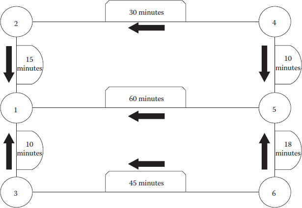
5.  Formulate and solve the network in Figure 7.30.

The solution is shown in Figure 7.31.

FIGURE 7.28
Exercise 7.1.

FIGURE 7.29
Exercise 7.2.

FIGURE 7.30
Exercise 7.5.

Solutions

1.  Objective MIN cost = MIN x₄₂c₄₂ + x₄₅c₄₅ + x₂₁c₂₁ + x₅₁c₅₁ + x₅₆c₅₆ + x₆₃c₆₃ + x₃₁c₃₁

Constraints

Node 1 : x₂₁ + x₅₁ + x₃₁ = 1 (because it is only one traveler)

Node 2 : x₄₂ = x₂₁

Node 3 : x₆₃ = x₃₁

Node 4 : x₄₂ + x₄₅ = 1 (one traveler)

Node 5 : x₄₅ = x₅₁ + x₅₆

Node 6 : x₅₆ = x₆₃

X_ij ≥ 0

2.  Objective MIN cost = MIN x₄₂c₄₂ + x₄₅c₄₅ + x₂₁c₂₁ + x₅₁c₅₁ + x₆₅c₆₅ + x₆₃c₆₃ + x₃₁c₃₁

Constraints

Node 1 : x₂₁ + x₅₁ + x₃₁ = 31 (because there are 31 in total)

Node 2 : x₄₂ = x₂₁

Node 3 : x₆₃ = x₃₁

Node 4 : x₄₂ + x₄₅ = 12

Node 5 : x₄₅ + x₆₅ + 6 = x₅₁

Node 6 : x₆₃ + x₆₅ = 13

X_ij ≥ 0

3.  Objective MIN cost = MIN x₂₄c₂₄ + x₅₄c₅₄ + x₁₂c₁₂ + x₁₅c₁₅ + x₆₅c₆₅ + x₃₆c₃₆ + x₁₃c₁₃

Constraints

Node 1 : x₁₂ + x₁₅ + x₁₃ = 1 (because it is only one traveler)

Node 2 : x₂₄ = x₁₂

Node 3 : x₃₆ = x₁₃

Node 4 : x₂₄ + x₅₄ = 1 (one traveler)

Node 5 : x₅₄ = x₁₅ + x₆₅

Node 6 : x₆₅ = x₃₆

X_ij ≥ 0

4.  

min(x_2,4 + x_2,5 + x_6,4 + x_6,5 + x_3,4 + x_3,5 + x_7,4 + x_7,5 + x_1,4 + x_1,5) − (q_1,4 = 1700)

5.  

FIGURE 7.31
Solution to Exercise 7.5.