We have taken an overview of mathematics in history. In this part of the book, we turn to two major subjects of mathematics, calculus and number theory, to be studied in detail. The first of these, calculus, is the focus of this chapter. Calculus has a rich historical tradition and is widely used in scientific endeavors today.
Calculus is the mathematics of change. It deals with rates of change of all kinds. We can use calculus to compute physical rates, such as the rate at which a rocket rises or a bomb falls, or the rate at which a radioactive substance decays. We can compute rates in biology, such as the rate at which a bacteria colony grows, the rate at which solutions diffuse across a membrane, or the rate at which a disease spreads through a population. It has applications in economics, such as marginal cost, marginal profit, and elasticity of demand. We use calculus to solve engineering problems, like how to make a roller coaster exciting but not dangerous.
Using calculus, we can maximize and minimize quantities. How can we produce a can of green beans in the most efficient way possible? Calculus is part of the answer. How can we maximize the profit of a company, or an industry, or an economy? Calculus plays a part in the models that answer these questions.
If something changes, and nearly everything interesting changes, calculus may have a role in describing it or modeling it.
A good way to begin learning calculus is to think about falling objects. Consider the simple question: A pencil falls from a four foot high counter; how fast does it hit the floor?
To answer this question, we might create an experiment where we carefully time a pencil as it falls. If we did that, we would find that it takes the pencil almost exactly one-half second to fall four feet. Knowing that rate is distance divided by time, we might then conclude that the speed of the pencil is
In practice, we try to be careful to measure distance by subtracting earlier positions from later positions. Since the height of the pencil at time zero was 4 feet and the height of the pencil after one-half second was 0 feet, we actually get the speed of the pencil to be
We use the word velocity to describe speeds when direction is important. In this case, the velocity is negative to indicate that the pencil is falling (i.e., moving in a downward direction).
A little more thought will convince us that this is not the right answer. Dividing total distance by total time gives us the average rate, the average velocity of the pencil. The pencil is barely moving when it first starts falling and then goes faster and faster under the influence of gravity. The average velocity (being somewhere in the middle) will be faster than the very slow speed at the beginning of the pencil’s descent and too slow to be the speed at which the pencil hits the floor.
Perhaps, if we had a quick eye, we could see where the pencil was after 1/4 seconds. If we had a very quick eye, we would know that after 1/4 seconds the pencil was still about three feet above the floor. Since it falls the last 3 feet in only 1/4 seconds, we could redo our calculation to get
This is better, but it is still too slow for the same reason that our first estimate was too slow (because we want the velocity at the bottom, not somewhere in the middle of the descent).
What if we could continue making estimates over shorter and shorter time intervals? Over a very short interval, there isn’t much time for the pencil to accelerate, so the average velocity and the velocity we want should be almost exactly the same.
It would take a fast eye to see where the pencil is 1/16 or 1/32 of a second before the pencil hits the floor, but a video camera takes pictures at a frame rate of one frame every 1/29.97 ≈ 0.03337 seconds. If we dropped our pencil on camera, we could flip through frames and discover these data points:
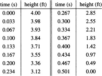
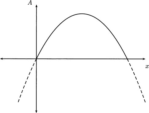
Graphically, the data look like Figure 4.1.
Figure 4.1 A graph of pencil heights over time.
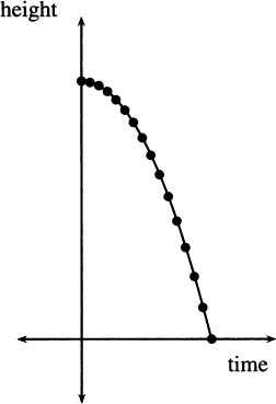
In 1638 Galileo asserted that the distance fallen is proportional to the square of time. Thus, the distance an object falls has an equation of the form d = kt2, where k is a constant. Because our data points show how high the pencil is (starting from a 4 foot counter), adapting Galileo’s idea, there should be a formula for our data that looks like y = 4 – kt2. Indeed, you can check by hand that these points are very closely predicted by the formula
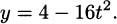
This is the formula for the curve shown connecting the dots on the previous plot.
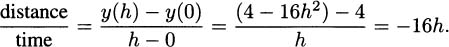
Once we know this formula, we can be as precise as we like about estimating the speed the pencil hits the floor. For example, the average speed during the last 1/16 seconds would be

We could continue to use shorter and shorter intervals, but that would mean repeating essentially the same computation over and over. We can save ourselves a lot of tedium by introducing a small bit of algebra. Let h be the length of the time interval we want to use (it could be the last 1/4 seconds, the last 1/16 seconds, or even smaller). Then the average speed of the pencil from time 0.5 – h to time 0.5 seconds is
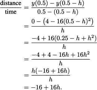
It is now quick work to calculate as many estimates of the pencil’s collision speed as we like.
| h | estimate |
| 0.5 s | –8 ft/s |
| 0.25 s | –12 ft/s |
| 0.0625 s | –15 ft/s |
| 0.01 s | –15.84 ft/s |
| 0.001 s | –15.984 ft/s |
As h gets smaller and smaller, it is apparent that –16 + 16h gets closer and closer to –16. This gives us the true answer to our question. Over any time interval, the average velocity of the pencil will be some number larger (i.e., less negative) than –16 ft/s. But as the time intervals become shorter and shorter, the average velocities get closer to –16 ft/s, the speed of the pencil the instant it hits the floor.
There was nothing particular about the time t = 0.5 except that it happened to be the time when the pencil hit the floor. We could just as easily have estimated the speed of the pencil at any other instant during the descent. For example, let’s check the speed of the pencil the moment it starts to fall, at time t = 0, by finding the average speed over the time interval [0, h].
In this case, as h gets smaller and smaller (closer and closer to zero) the average speed goes to 0. This agrees with our intuition. Just for an instant when the pencil starts falling, it isn’t moving at all. Its instantaneous velocity at time 0 is 0 ft/s.
4.1 Find the instantaneous velocity of a pencil dropped from a height of 4 ft when t = 0.25 s, i.e., the moment its height is 3 ft.
4.2 An object dropped from a height of 16 ft takes approximately one second to strike the ground, and it has a height function of y = 16 – 16t2.
4.3 A more precise height function for a pencil dropped 4 feet is y = 4 – 16.1t2. It only takes about 0.49844 seconds (not a full half second) for the pencil to reach the floor.
4.4 If your home were on the Moon, and a pencil were to drop 4 ft to the floor, its height function in feet would be y = 4 – 2.65t2.
4.5 A person shoots an arrow vertically into the air at 200 ft/s. Neglecting air resistance, the height of the arrow after t seconds is given by the formula y = 6 + 200t – 16.1t2 (approximately).
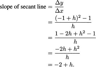
If we think about the process we developed in Section 4.2, each time we chose a time interval and computed the average velocity of the pencil over the interval, we were finding a value that looked something like
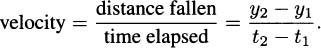
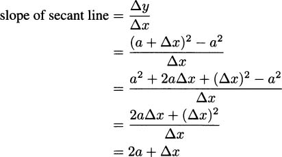
Considering the problem geometrically (looking at the graph of what we are doing), we can see that the key to the whole process is slopes. Since slope is the ratio of the change in the y-coordinates (the rise) to the change in the t-coordinates (the run), we can write slope as Δy/Δt. (The Greek letter delta, Δ, stands for change.) Each of these average velocities is the slope of some line intersecting the height function at two points. See Figure 4.2.
We saw that finding the instantaneous velocity amounted to a limiting problem where Δt, which we called by the name h, was allowed to get closer and closer to zero. In the picture, we interpret this as a question about the slopes of lines that intersect a function when the points of intersection are brought closer and closer together. Each average velocity for the pencil is the slope of some line through the curve, so if we want to know about the (instantaneous) velocity of the pencil, we can focus our attention on slopes of lines.
A tangent line to a curve is a line that touches the curve in just one point, and closely approximates the curve near that one point. In Figure 4.3, a tangent line is drawn touching the curve where t = 1/2. Notice that the tangent line looks very much like the limit of the lines in Figure 4.2 when Δt approaches zero.
Figure 4.4 shows a general curve and a tangent line to the curve at a point P on the curve.
To find tangent lines in general, we use our experience with instantaneous velocities for inspiration. To find the tangent line at P in Figure 4.5, we begin by putting a second point Q on the curve somewhere nearby. We can put Q pretty much any where on the curve to start out, though often you’ll pick somewhere near P. The line through P and Q is called a secant line.
Figure 4.2 Average velocities are slopes of lines.
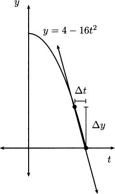
Figure 4.3 A tangent line is the key to instantaneous velocity.
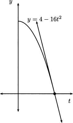
Figure 4.4 A curve and its tangent line.
Figure 4.5 Tangent lines are derived from secant lines.

Now, if Q gets closer and closer to P (which is what happened when we observed our pencil over shorter and shorter time intervals), then the secant line through P and Q becomes a better and better approximation to the tangent line at P. If we can make Q coincide with P, by using a limiting process, then the secant line will “become” the tangent line at P. This is good for us, since the slope of the tangent P is going to tell us how fast our pencil hits the floor.
In the following examples, we will refer to P (the point where the tangent line touches the curve) as the base point. We will refer to Q as the second point.
The method of using a limiting process of secant lines to find a tangent line was discovered by Pierre de Fermat (1601–1665). It was expanded upon by the two discoverers of calculus, Isaac Newton (1642–1727) and Gottfried Wilhelm von Leibniz (1646–1716).
 EXAMPLE 4.1
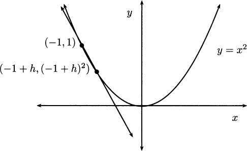
We will find an equation of the tangent line to the parabola y = x2 at the point (–1, 1). The base point is (–1, 1). We take the second point to be (–1 + h, (–1 + h)2), where h is an arbitrary nonzero number. In Figure 4.6, h is positive, so the second point is to the right of the first point. But h could just as well be negative, with the second point to the left of the base point. The calculations work the same either way.
Figure 4.6 Tangent to y = x2.
When h diminishes to 0, we obtain the slope of the tangent line:

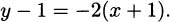
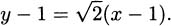
We have a slope, –2, and a point, (–1, 2), so we can use the point-slope form of a line, y – y0 = m(x – x0), to describe the tangent. Thus, an equation of the tangent line to y = x2 at the point (–1, 1) is
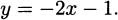
If we want to solve this equation for y to put the line in the more familiar y = mx + b form, we can:
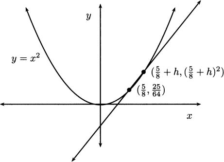
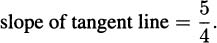
EXAMPLE 4.2Let’s find an equation of the tangent line to the parabola y = x2 at the point  (see Figure 4.7).
Figure 4.7 Tangent to y = x2 at .
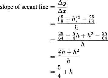
When h diminishes to 0, we obtain the slope of the tangent line:
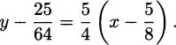
Using the point-slope form again, an equation of the tangent line is
Looking over the last two examples, we see that the slope of the tangent line to the curve y = x2 at the point (–1, 1) is –2, and the slope of the tangent line to the same curve at the point is  . In both cases, the slope of the tangent line is double the value of the x coordinate. Let’s use the next example to show that this is always the case for the curve y = x2.
EXAMPLE 4.3Let’s find the slope of the tangent line to the parabola y = x2 at the point (a, a2), where a is an arbitrary number (Figure 4.8). Based on our previous work, we expect that our answer is going to be 2a.
This time, for variety, we choose to write Δx for h.
Figure 4.8 Finding the slope at an arbitrary value a.
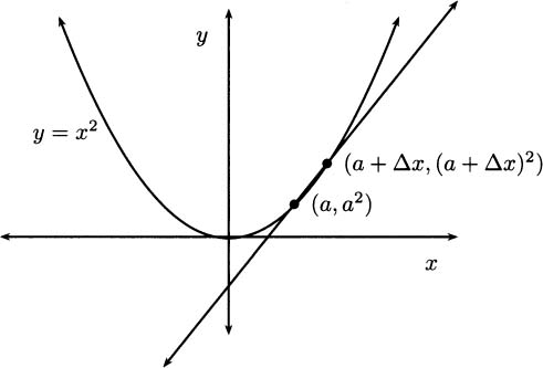
When Δx diminishes to 0, we obtain the slope of the tangent line:

Notice that if we let a = – 1, then we find the slope of the tangent line at (–1, 1), and we get the same answer, –2, as we got in Example 4.1. If we let a = 5/8, we get the same answer, 5/4, that we got in Example 4.2.
4.6 Use the secant line method to find an equation of the tangent line to the parabola y = x2 at the point (3,9).
4.7 Use the secant line method to find an equation of the tangent line to the parabola y = x2 at the point (–4, 16).
4.8 Use the secant line method to find an equation of the tangent line to the parabola y = 4 – 16t2 at the point (0.25, 3).
4.9 Find the slope of the tangent line to the parabola y = 4 – 16t2 at an arbitrary point (a, 4 – 16a2). The slope of this tangent corresponds to the velocity of our falling pencil in Section 4.2. Use this slope to determine the velocity of the pencil when t = 0.0, 0.1, 0.2, 0.3, 0.4, and 0.5 seconds.
4.10 Find the slope of the tangent line to the parabola y = 16 – 16t2 at an arbitrary point (a, 16 – 16a2). The slope of this tangent corresponds to the velocity of a pencil dropped from a height of 16 feet. Use this slope to determine the velocity of the pencil when t = 0.0, 0.25, 0.5, 0.75, and 1.0 seconds.
4.11 Find the slope of the tangent line to the parabola y = 4–2.65t2 at an arbitrary point (a, 4–2.65a2). The slope of this tangent corresponds to the velocity of a pencil dropped from a 4 foot desk on the Moon. Use this slope to determine the velocity of the pencil when t = 0.0,1, and 1.2286 seconds.
4.12 If your home were on Mars, the height function of a pencil dropped from a 4 foot desk would be the parabola y = 4 – 6.12t2.
Recall from algebra class the definition of a function. A function is a rule that assigns to each number x in some domain exactly one number y in a range. For example, y = x2 describes a function by giving a formula. The domain of the function is the set of values you can “put in” the function, all real numbers in this case (since every number can be multiplied by itself). The range is the set of values that you “get out” of the function, and for the squaring function this is the set [0, ∞). You probably remember many happy hours spent finding the domains and ranges of functions.
In addition to having a domain and range, we know that y = x2 describes a function because for any x we put in we get out exactly one y. If x = 3 goes in, y = 9 comes out. Put in x = 0 and you get out y = 0, etc. There is only one way to square a number.
You may remember that functions have graphs that pass the vertical line test. This is the same thing; at any particular x-value, the function should only have a single y-value (which is where it intersects the vertical line).
Not all formulas describe functions. For example, y = x1/2 is not a function, because if you put in x = 9, the value for y is ambiguous. It could be y = 3 or y = – 3. However, usually when we write y =  we mean the positive square root; and this is a function, because there is only one way to find a positive square root.
In Example 4.3 we saw a process that can unambiguously tell us the slope of a tangent line at any point on a curve. That is, there is a formula that can tell us slopes when given x-values. If you name an x-value, I can tell you the slope. Name a different x-value, and I can tell you the new slope.
Since the slope of a tangent line is a rule we can give unambiguously, we know from our experience in algebra that it is a function, and this function has a name. It is called the derivative. Sometimes people refer to the derivative as the “slope generating function.”
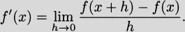
The process of finding the derivative of a function is called differentiation. The notation f′(x) is read “f prime of x.”
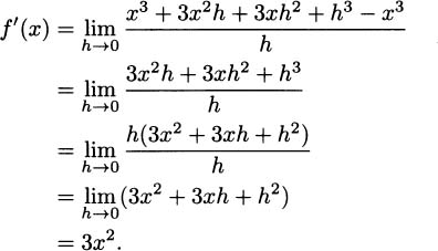
EXAMPLE 4.4Let’s find the derivative of f(x) = x3. According to our definition,
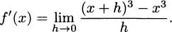
Using the expansion (x + h)3 = x3 + 3x2h + 3xh2 + h3, we have
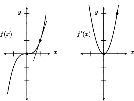
We can use this new function to find the slope of the tangent line at any point on x3. For example, when x = 0, the slope is f′(0) = 3(02) = 0. Likewise, when x = 1, the slope is f′(1) = 3(12) = 3. This is represented visually in Figure 4.9.
Figure 4.9 Graphs of f(x) and the derivative f′(x).
4.13 Use the definition to find the derivative of the function f(x) = x2 + 3. Draw a sketch of f(x), or graph it on a calculator, and check that the slopes given by f′(x) look right.
4.14 Use the definition to find the derivative of the function f(x) = x2 + 5. Draw a sketch of f(x), or graph it on a calculator, and check that the slopes given by f′(x) look right.
4.15 Use the definition to find the derivative of the function f(x) = x2 + x. Draw a sketch of f(x), or graph it on a calculator, and check that the slopes given by f′(x) look right.
4.16 Use the definition to find the derivative of the function f(x) = 3x. Draw a sketch of f(x), or graph it on a calculator, and check that the slopes given by f′(x) look right.
4.17 Use the definition to find the derivative of the function f(x) = 3x + 1. Draw a sketch of f(x), or graph it on a calculator, and check that the slopes given by f′(x) look right.
4.18 Use the definition to find the derivative of the function f(x) = –2x + 2. Draw a sketch of f(x), or graph it on a calculator, and check that the slopes given by f′(x) look right.
4.19 Use the definition to find the derivative of the function f(x) = x3 + x. Draw a sketch of f(x), or graph it on a calculator, and check that the slopes given by f′(x) look right.
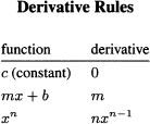
We saw in Section 4.3 that slopes can be used to compute tangible things such as velocities of objects. In Section 4.4 we created a formal mathematical process for finding slopes, called differentiation. Since derivatives are the key to solving all kinds of mathematical problems, it is natural to want to know the derivative of as many different kinds of functions as possible. However, even the most mathematical of us eventually find it tedious to compute derivatives using the limit definition. Luckily, there are easily recognizable patterns that we can use as shortcuts, or “derivative rules.”
The simplest derivative rule is that the derivative of a constant function f(x) = c is f′(x) = 0. The graph of a constant function f(x) = c is a horizontal line that intersects the y-axis at the value c. Since it is a horizontal line, it has a slope of 0 everywhere. That is, at every x the slope is zero. This is precisely what f′(x) = 0 means (it gives 0 for every value of x).
Non-horizontal lines are just as easy. The derivative of a linear function f(x) = mx is f′(x) = m, since f is a line through the origin with slope m. Of course, nothing changes if the y-intercept happens to be different from 0 (i.e., if the line doesn’t go through the origin); it still has slope m. We can write this idea as a rule, and we have our first rule of derivatives.
The line rule: If f(x) = mx + b, then f′(x) = m.
Notice that the line rule contains the constant rule within it. If f(x) = b is a constant function, then the line rule tells of that f′(x) = 0. For example, if f(x) = 7 = 0x + 7 is a horizontal line (with y-intercept 7), then its derivative is zero.
EXAMPLE 4.5We can check the line rule carefully, using the definition of derivative. If f(x) = mx + b, then the definition of derivative tells us that
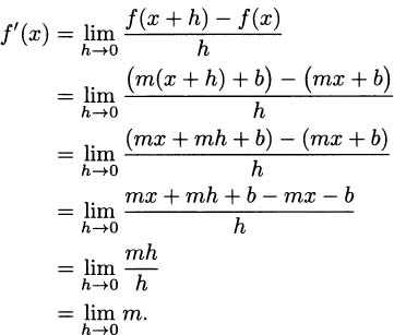
It feels a little strange to ask what m is getting close to as h becomes closer and closer to 0, since m is just a number, but it’s perfectly correct to declare that it gets close to m. You might say that being exactly equal to something is the very best way to get close to it.
So we get f′(x) = m. Of course, a slope of m is exactly what our experience tells us to expect for the line f(x) = mx + b.
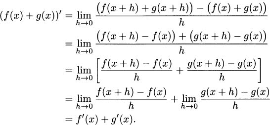
It might have occurred to you that the function f(x) = mx + b is actually the sum of two lines, a non-horizontal line g(x) = mx and a horizontal line h(x) = b. Using the line rule for each, we get g′(x) = m and h′(x) = 0. Notice that if we add these derivatives, g′(x) + h′(x) = m, which happens to be the same as f′(x). This is not a coincidence, but is our second rule of derivatives.
The sum rule: The derivative of a sum is the sum of the derivatives:
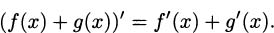
EXAMPLE 4.6Since 3x = 2x + x, we can use the line rule directly to determine that (3x)′ = 3, but we can also use the sum rule (and the line rule) on the right hand side to get (3x)′ = (2x)′ + (x)′ = 2 + 1 = 3. It doesn’t matter which rules we use, we always get the same answer for the derivative.
If your algebra skills are good, you can verify the sum rule using the limit definition:
EXAMPLE 4.7The sum rule works for three (or more) terms as well. For example, take f(x) = x + x + x. We can group with parentheses, to make this a sum of just two terms, f(x) = x + (x + x). Then an application of the sum rule tells us
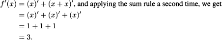
The key observation is that this pattern always works, no matter what functions you use. So (f(x) + g(x) + h(x))′ = f′(x) + g′(x) + h′(x).
In Example 4.4 we discovered that (x3)′ = 3x2. Before that, in Example 4.3 we determined that (x2)′ = 2x. The line rule tells us that (x1)′ = 1, since x1 is another way of writing x. And because x0 = 1 we can see that (x0)′ = 0. Perhaps you have already determined that these all adhere to a common pattern.
The power rule: For any integer n ≥ 0, the derivative of the power function f(x) = xn is f′(x) = nxn–1.
EXAMPLE 4.8Let’s find the derivative of f(x) = x10. By the power rule, we have
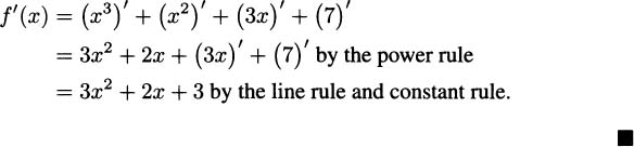
EXAMPLE 4.9Find the derivative of f(x) = x3 + x2 + 3x + 7.
Solution: By the sum rule, we have
There is a straightforward differentiation rule for multiplying functions by constants.
The constant coefficient rule: If c is a constant, then (cf(x))′ = cf′(x).
In terms of the graph, multiplying a function by some constant has the effect of stretching (or compressing) it vertically. For example, the function f(x) = 2sin x is twice as tall as a standard sine curve. What the constant coefficient rule tells us is that the coefficient applies to slopes in the same way. Examine Figure 4.10 to see that this seems plausible.
Figure 4.10 Slopes on 2 sin x are twice the size of slopes on sin x.
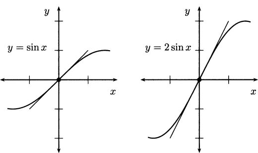
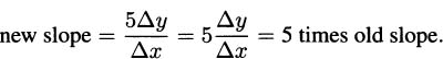
Intuitively, slope is always a calculation of “rise over run.” If we multiply a function by the constant 5, then in slope calculations the “rise” changes by the same factor of 5 (because all of the y-values are 5 times as large), but the “run” is the same. The new slope would look something like
This agrees with what we already know from the line rule. By the line rule, we know that the derivative of 7x is 7. The constant coefficient rule tells us that we can also think of it as 7 times the derivative of x. Of course 7(x)′ = 7 · 1 = 7, so we get the same answer.
In the same way, the constant coefficient rule tells us that (5x3)′ = 5(x3)′ = 5 · 3x2 = 15x2.
The power rule, sum rule, and constant coefficient rule combine to tell us everything we need to take the derivative of any polynomial. At first, we should probably compute derivatives step by step, but soon we’ll be taking derivatives almost effortlessly.
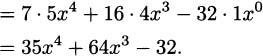
EXAMPLE 4.10Let’s find the derivative of f(x) = 7x5 + 16x4 – 32x + 100. By the sum rule, we know that

The constant rule tells us that (100)′ = 0, and the constant coefficient rule lets us “pull out” the constant from each of the other terms we are taking the derivative of, so

Finally, applying the power rule,
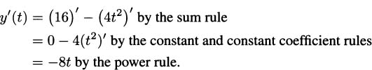
EXAMPLE 4.1lWhile we are building these differentiation rules, we should not get caught up in the letters we use. Functions do not have to be called f and their variable does not have to be x. The rules apply in the same ways if we use other variable and function names. For example, the derivative of y(t) = 16 – 4t2 is
Here is a summary of some important derivative rules:
4.20 Use derivative rules to verify the derivatives we found for each of the functions from the previous exercise set.
4.21 Find the derivative of each polynomial.
4.22 The parabola y = x(x – 1) = x2 – x has a single point where the slope is 0. Find the value of x where the slope, i.e., the derivative, is 0. Then find the corresponding y. (The point (x, y) identifies the vertex of the parabola.)
4.23 The function y = x3 – x has two points where the slope is 0. Find both. Sketch the graph of the function by plotting points or using a calculator, and verify that the tangent line looks horizontal at both points.
4.24 Use derivative rules to find an equation of the tangent line to the parabola y = 3 – x2 at the point (1,2). (Hint: you are given a point, and the derivative tells you the slope.)
4.25 A pencil dropped from a height of 4 feet has a height function that looks like y(t) = 4 – 16.1t2. It only takes about 0.49844 seconds (not a full half second) for the pencil to reach the floor.
4.26 A pencil thrown vertically into the air from a height of 4 feet has a height function that looks like y(t) =4 + 5t – 16.1t2.
Say we have two functions, f(x) and g(x). If we knew that the derivative of f(x) was 6 and the derivative of g(x) was 5, what would be the derivative of the product f(x)g(x)?
If you answered 30, you are probably not alone. But unfortunately you’re not right either, and you can easily check for yourself that this is a mistake. You could, for example, take f(x) = 6x. That’s a function with f′(x) = 6. If you also take g(x) = 5x, then g′(x) = 5. And when we multiply? We get f(x)g(x) = 6x · 5x = 30x2. This means that the derivative of the product f(x)g(x) is then the derivative of 30x2, and that is 60x, and not 30.
It turns out that there is a product rule for derivatives, but it is not the naively simple rule that most people guess.
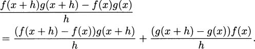
The product rule: If we can compute the derivatives of f(x) and g(x), the derivative of their product is (f(x)g(x))′ = f′(x)g(x) + f(x)g′(x).
EXAMPLE 4.12If we take f(x) = 6x and g(x) = 5x, then the product rule tells us that
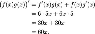
Naturally, this is the same as the answer we get without the product rule (when we do it correctly).
EXAMPLE 4.13What is the derivative of

Solution: In plain English, the product rule tells us, “the derivative of a product is ‘the derivative of the first’ times ‘the second’ plus ‘the first’ times ‘the derivative of the second.’” Computing, we have
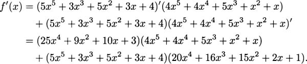
This may seem like an unsatisfyingly complicated answer, but it would be completely adequate if we were in a situation where we didn’t need to simplify. Although we devote extensive effort in algebra class to simplification, we don’t always need to simplify to solve problems. For example, if all we need to know is the slope of f when x = 0, it is straightforward to find that f′(0) = (3)(0) + (4)(1) =4, and the computation is easy even without simplifying.

EXAMPLE 4.14We can use the product rule when there are more than two factors. We simply apply the product rule more than one time. Consider the function h(x) = x(x + 1)(x + 2). Although this function is easy to handle by multiplying things out, let’s use the product rule instead.
To get started, we have to decide which factors of the function will constitute the f(x) part of the product rule and which factors will be the g(x) part. It doesn’t really matter, as long as you split the function into two factors that are multiplied together. Let’s choose f(x) = x(x + 1) and g(x) = x + 2. Then h(x) = f(x)g(x), and we can differentiate:
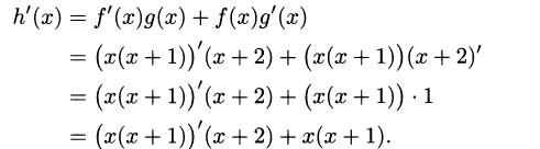
For the derivative of x(x + 1), we use the product rule a second time. Continuing,
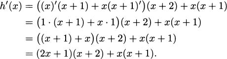
If we wish to combine terms and simplify a bit, we conclude that h′(x) = 3x2 + 6x + 2. Of course, this is the same answer that we get if we multiply h out first and differentiate directly.
Naturally, we can differentiate functions that are products of four factors (it requires three applications of the product rule), or five factors, or more.
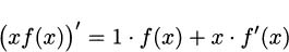
We can use the product rule to figure out the derivatives of functions we don’t yet know how to differentiate. For example, what is the derivative of f(x) = 1/x? We can use the product rule, if we are careful and clever.
If we start with f(x) – 1/x, then xf(x) = 1, which is a constant. Constant functions are easy to differentiate, so we know immediately that (xf(x))′ = 0. But we can also find the derivative using the product rule. According to the product rule,
Putting these two calculations together (remembering that f(x) = 1/x), we get
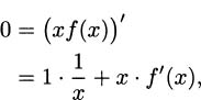
and it follows that
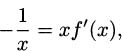
and finally that
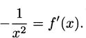
So if f(x) = 1/x, the derivative is f′(x) = –1/x2.
The previous argument is an example of a common proof method in mathematics. If we can compute a quantity two different ways, then we know both answers must be equal even if they may not look the same. As in this discussion, often the clever step is figuring out how to arrange things (i.e., knowing to start with xf(x) = 1 and then differentiate). Once arranged, the calculations are not necessarily difficult.
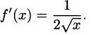
EXAMPLE 4.15Find the derivative of f(x) = .
Solution: We need to arrange things so we can use the product rule, so let h(x) = f(x)f(x) = = x. We can immediately see that h′(x) = 1, but we can also apply the product rule. This means that
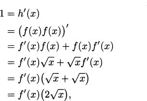
and dividing, we have
Just as we can find the derivative of products of functions, there is a rule for taking the derivatives of quotients of functions (that is, when we divide functions). The quotient rule is not easily guessed, but amazingly we can figure out the formula using the product rule.
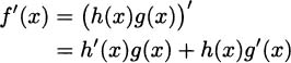
First we need a quotient. Let h(x) =  . Our goal is to find a formula for h′(x). When we cross-multiply, we get h(x)g(x) = f(x), or reversing the equality we have f(x) = h(x)g(x), and this is a product, so we can differentiate it. On the left, we’ll simply write the derivative as f′(x). On the right, we’ll use the product rule.
Now, keep the term with h′(x) on the right, and move everything else to the left side.

Reverse the equality and divide by g(x) to get h′(x) alone.
Next comes a clever part, but we’re almost finished. Remember that we started with h(x) = . Substitute for h(x) to get
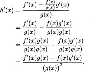
This becomes our rule for differentiating quotients.
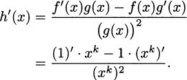
The quotient rule: If h(x) = , then h′(x) =  .
.
Because this formula is fairly complex, people usually use one of two ways to remember it. In words we say that the derivative of a fraction is, “Bottom times the derivative of the top, minus top times the derivative of the bottom, all over the bottom squared.”
Some people prefer to remember the quotient rule via the (math) poem,
Read aloud, this goes, “Low dee-high, minus high dee-low, over low low (and away we go)!” In the poem, low refers to the bottom function g(x), high refers to the top function f(x), and dee reminds us to take a derivative. So ‘low dee-high" is g(x)f′(x). Similarly, “high dee-low” is f(x)g′(x). And we divide by “low low,” which is g(x) · g(x) = (g(x))2. If you write everything out according to the poem, you get the quotient rule.
EXAMPLE 4.16Let us apply the quotient rule to a function we already know the derivative of, such as x2.
We can think of h(x) = x2 as a quotient by writing it as h(x) =  . Then, for the purposes of applying the quotient rule, f(x) = x2 and g(x) = 1. We calculate

which we know is correct.
EXAMPLE 4.17Find the derivative of h(x) = 1/xk where k is a positive integer (1, 2, 3, etc.).
Solution: Take f(x) = 1 and g(x) = xk. By the quotient rule,
Here we can use the power rule to continue.
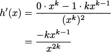
To divide powers, we subtract exponents.

This completes the power rule. The computation we just finished verifies that the derivative of x–k is –kx–k–1. In other words, the power rule works with negative exponents. We now state the general power rule.
The power rule: If n is any integer (positive, negative, or zero), the derivative of the power function f(x) = xn is f′(x) = nxn–1.
EXAMPLE 4.18Find the derivative of h(x) =  .
.
Solution: By the quotient rule,
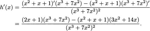
At this point, you may be inclined to simplify, but you should probably consider whether this gains you much. For example, if you merely need the slope of the function when x = 1, it is probably easier to evaluate h′(1) directly without simplifying. You’ll be less likely to make an error.
In this example, our goal was simply to find the derivative. We have done that, so we’ll stop here.

4.27 Calculate the derivative of each function, once by multiplying out and also using the product rule. Verify that you get the same answer either way.
4.28 For each function in the previous exercise:
4.29 Differentiate h(x) = x(x + 1)(x + 2) as we did in Example 4.14, only this time take f(x) = x and g(x) = (x + 1)(x + 2) as your factors for the product rule. Verify that you get the same answer.
4.30 Differentiate h(x) = x(x + 1)(x + 2)(x + 3) with the product rule.
4.31 Use the product rule to find the derivative of f(x) = 1/x2. (Hint: start with x2f(x) = 1.)
4.32 Use the product rule to find the derivative of f(x) =  .
.
4.33 Use the product rule to find the derivative of f(x) =  .
.
4.34 Find the derivative of each quotient,


4.35 For each function in the previous exercise:
4.36 Find the derivative of each.

4.37 Show why the product rule is true. Hint:
The sum rule allows us to take the derivative of f(x) + g(x). The product rule tells us how to differentiate f(x)g(x), and the quotient rule lets us take the derivative of . But there is another way we can combine functions, one that we haven’t yet discussed.
Can we take the derivative of a composition of functions? If h(x) = g(f(x)), is there a way to say what the derivative will be? For example, if f(x) =  and g(x) = x2 then
Is there a way to compute the derivative of h, a way that lets us use what we know about f and what we know about g? It turns out that there is. It’s called the chain rule.
The chain rule: If h(x) = g(f(x)), then h′(x) = g′(f(x))f′(x).
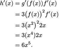
EXAMPLE 4.19Find the derivative of h(x) = (x2)3.
Solution: By properties of exponents, h(x) = x6, and the power rule directly tells us that h′(x) = 6x5. We can also use the chain rule to arrive at this. For the purposes of the chain rule, the “inside” function of the composition is f(x) = x2. The “outside” function is g(x) = x3.
By the power rule, f′(x) = 2x and g′(x) = 3x2, and according to the chain rule,
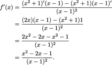
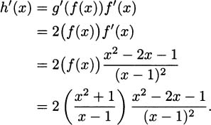
EXAMPLE 4.20Let’s apply the chain rule to h(x) =  . Here f(x) = and g(x) = x2. The derivative of g is easy: g′(x) = 2x. For the derivative of f, we use the quotient rule:
According to the chain rule, the derivative of h is
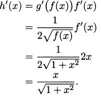
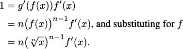
EXAMPLE 4.21In Example 4.15 we showed that the derivative of g(x) = is g′(x) =  . Find the derivative of h(x) =
  .
.
Solution: In this case, the inside of the composition is f(x) = 1 + x2, and the outside is g(x) = . By the chain rule,
If fractional exponents are a dim memory for you, remember that a square root can be written as an exponent of 1/2. This is not crazy. Just as you multiply by itself to get x, when you multiply x1/2 · x1/2 you get x1 by adding exponents.
In Example 4.15 we used the product rule to find the derivative of , that is, the derivative of the function y = x1/2. Knowing the chain rule, we can find the derivative of any root.
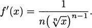
Let f(x) =  = x1/n, where n is a positive integer (1, 2, 3, …). If we take the nth power of both sides, we learn that (f(x))n = x. Now, x is something we know the derivative of, and its derivative is 1. The left side of the equality is a composition, however, and we can apply the chain rule.
For the purposes of the chain rule, the outside function is g(x) = xn. The inside function is f(x). Taking the derivative, we get
It’s really f′ that we are interested in, and solving for f′, we get
If we use fractional exponents for the root, we can make this a bit simpler:
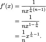
Thus, the chain rule tells us that the derivative of f(x) = x1/n is  . This is exactly as we might have guessed from the power rule.
EXAMPLE 4.22If f(x) = = x1/2, then  . This agrees with our conclusion in Example 4.15.
EXAMPLE 4.23Find the derivative of h(x) = x2/3.
Solution: We can write  . This is a composition of two functions. The outside function is g(x) = x1/3, and the inside function is f(x) = x2. By the chain rule,
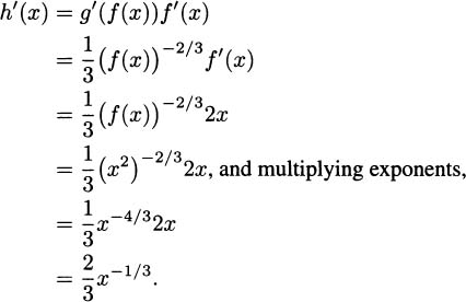
Notice that this agrees with the pattern of the power rule. The derivative of h(x) x2/3 is  .
.
It turns out that the power rule works for any fractional exponent. Although we don’t prove it here, the power rule works for all exponents, even irrational ones.
The power rule: If f(x) = xr, where r is any real number, then f′(x) = rxr–1.
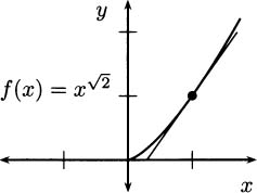
EXAMPLE 4.24Find the tangent to  when x = 1.
Solution: To find a tangent line, we need two pieces of information, the point of tangency and the slope of the line. When x = 1, we have y = f(1) =  = 1, so the point of tangency is (x, y) = (1, 1).
The derivative of the function tells us the slope of the tangent, and the derivative of is simply  . When x = 1, the slope is f′(1) =
  .
.
Putting these together using the point-slope form of a line, we obtain the tangent line
If you prefer the y = mx + b form of a line, you can simplify to get
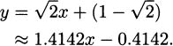
A plot on a calculator or computer, like Figure 4.11, can help us verify that this answer is correct and we have made no mistakes.
Figure 4.11 Tangent to the power function  .
.
4.38 Find the derivative of each function:

4.39 For each function in the previous exercise:
In calculus, the term optimization refers to finding the maximum or minimum of some quantity. The maximized quantity can refer to something physical, like the maximum height of a ball thrown into the air. Or it can be non-physical, like the production level of a manufacturing plant that maximizes profit for the company (or minimizes cost).
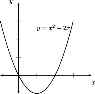
Consider the parabola f(x) = x(x – 2) = x2 – 2x in Figure 4.12.
From the graph, it seems obvious that the function has a minimum occurring between x = 0 and x = 2. You may even intuitively guess that the smallest value happens precisely at x = 1. Let’s use calculus to verify this.
Figure 4.12 Finding the minimum of a parabola.
The key to finding a minimum is to consider slopes, which means we want to use the derivative function. For this parabola, the derivative is f′(x) = 2x – 2.
Observation 1: If the derivative is negative, then the slope of the function is “down” and the function gets smaller (or more negative) as we move to the right. A point where the slope is negative is not going to be a minimum because we can move a little bit to the right and find smaller function values.
When is f′(x) = 2x – 2 negative? Compute:

For any value x < 1 we know that the derivative is negative and, consequently, f(x) gets smaller as we move to the right. In mathematical language, we say f(x) is decreasing. No x on the left side of 1 can possibly be a minimum of f. Look at the graph, and see that this makes sense.
Observation 2: If the derivative is positive, then the slope of the function is “up” and the function gets bigger (or less negative) as we move to the right. A point where the slope is positive is not going to be a minimum because we can move a little bit to the left and find smaller function values.
When is f′(x) = 2x – 2 positive? Compute:
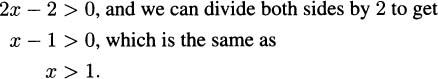
For any value x > 1 we see that f(x) gets larger as we move to the right, and smaller as we move to the left. In mathematical language, we say f(x) is increasing. No x on the right side of 1 can possibly be a minimum of f. Look at the graph, and see that this makes sense.
Putting these two observations together, we now can be certain that x = 1 is the location of a minimum of f, for f is decreasing when x < 1 and increasing when x > 1.
The value x = 1 is the location of the minimum. If we were asked to find the minimum value of the function, we would want to put that value back into f to find the y-value. For this parabola, the minimum value would be f(1) = 12 – 2 · 1 = – 1. If we were asked to give the lowest point on the function, we should give the ordered pair for the point, (x, y) = (1, –1).
Given a function f(x), we are interested in places where f may have a maximum or minimum. In general, functions may have no maximum or minimum, or they may have one or two or possibly many maxima and minima. So far, we have discovered that f′(x) > 0 guarantees that x is not the location of a max or min. We also have seen that f′(x) < 0 guarantees that x is not the location of a max or min.
Where then should we look for maxima and minima? Author William Priestley suggests we should think about such problems like Sherlock Holmes.1 There is a famous Holmes quote that reads, “When you have eliminated the impossible, whatever remains, however improbable, must be the truth.” We have seen that a max or min is impossible where the derivative is either positive or negative. According to Sherlock Holmes, we eliminate these places and look for maxima and minima at the points that remain, i.e., at the places where the derivative is not positive or negative.
Critical points are not always maxima and minima, but if we follow the thinking of Sherlock Holmes they are the right places to look for maxima and minima. In mystery parlance, you might call them suspects. They are the places we suspect to find maxima and minima.
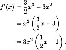
EXAMPLE 4.25Let  . Find any maxima or minima.
Solution: To check for critical points, we take the derivative:
There are two ways a critical point can occur: the derivative can be zero or it can be undefined. In this example, the derivative is a polynomial, so there is no way for it to be undefined (we’ll never divide by zero, take the square root of a negative, etc.).
So we can focus on zeros. This is why we factored the derivative. It makes finding zeros simpler. If we set f′(x) = 0, we can see that either 3x2 = 0 or  x – 1 = 0. Consider each, in turn. If 3x2 = 0, then x = 0. If x – 1 = 0, then x = 2.
So the function f has critical points when x = 0 or when x = 2. Accordingly, these are places to look for maxima and minima. Let’s consult a graph of f (Figure 4.13).
Figure 4.13 Checking the critical points at x = 0 and x = 2.
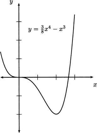
It would appear that x = 2 is the location of a minimum of f, but x = 0 is neither a maximum nor a minimum. When x = 0, the slope of the tangent line momentarily becomes zero (that is, horizontal). It looks like the function decreases on the left side of x = 0, becomes momentarily horizontal, and continues decreasing to the right until it reaches a minimum at x = 2.
We can verify the maxima and minima of a function in practice by checking the function value at a critical point and comparing to function values on both sides. Even without the graph, we could check:
| x | f(x) |
| –0.1 | .001 |
| 0 | 0 |
| 0.1 | –.001 |
| 1.9 | –1.972 |
| 2 | –2 |
| 2.1 | –1.968 |
As the graph indicates, the function is a bit positive when x = –0.1 and a bit negative when x = 0.1, telling us that (x, y) = (0,0) is a critical point that is not a max or min. However, when checking around x = 2, we see that the function is larger (that is, less negative) on both sides, verifying that x = 2 is the location of a minimum.
Our conclusion is that the minimum value of f is –2, which occurs at the point (x, y) = (2, –2). There are no maxima.
EXAMPLE 4.26Find the maxima and minima of f(x) =  .
.
Solution: To check for critical points, we take the derivative. We can either use the chain rule, thinking of f as a composition of functions, or we can first switch to fractional exponents.
Using fractional exponents, a cube root is the same as an exponent of 1/3, so  . (Remember that you multiply exponents when taking a power of a power.) So, the derivative is
  .
.
Critical points occur where the derivative is not positive and not negative. We need to look for values of x with either f′(x) = 0 or where f′(x) does not exist.
We can readily see that there are no values that make the derivative zero. The function f′ is a fraction, and fractions can only be zero when the numerator (top part) is zero. However, there is one value of x that makes the derivative undefined, x = 0, since we can’t divide by zero. So x = 0 marks a critical point.
We know from the previous example that a critical point may not actually indicate a max or min, so we’ll check the values of the function on each side:
| x | f(x) |
| –0.1 | .215 |
| 0 | 0 |
| 0.1 | .215 |
The critical point at x = 0 is apparently a minimum of f, because the values of the function are greater on both sides. Let’s compare with the graph in Figure 4.14.
Figure 4.14 Checking the critical point at x = 0.
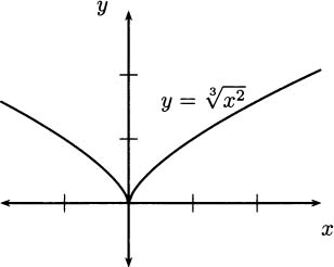
Our graph confirms that x = 0 is the location of a minimum of f. The graph also helps us visualize what occurs. At the origin, the tangent line to f becomes vertical, and you may recall that vertical lines have undefined slope (they are the only lines that cannot be written as y = mx + b, because there is no m).
The sharp point where the derivative becomes undefined is called a cusp, and this cusp forms a minimum for f. The function f has no maximum points.
In summary, optimization problems are solved by computing the derivative. Points where the derivative of a function is positive or negative will not be maxima or minima. If we eliminate these points, the remaining points are called critical points. Critical points occur where the derivative is zero or undefined and may or may not mark maxima and minima. We have to check each critical point in turn to see what kind of point it is.
4.40 Find the maxima and minima of each function. Compare with a graph to confirm your answers.
 x4 – 4x3 + 6x2
I have 200 m of fencing available to create a rectangular pen to hold some sheep. What is the largest area of grass that can be enclosed by my fence? We can use calculus to find the answer.
The key to solving an applied optimization problem is to find a way to model the situation with a function. We know we can use derivatives to optimize functions, that is, to find maxima and minima. To get started with the correct function, it helps to begin with the proper question.
What is it that we are trying to maximize or minimize?
In this case, we want to maximize the area of grass enclosed by the rectangular sheep pen. We need a function that represents the area, and then we can apply calculus.
Figure 4.15 A sheep pen.
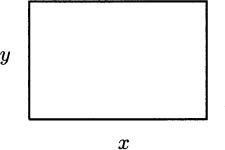
It is usually a good idea to draw a picture and label it, like Figure 4.15. Taking this as our picture, the area of the pen is simply

We would almost be ready to apply calculus, except for one impediment. The functions we have worked with so far have only one variable, but our area is in terms of both x and y. So there is one more step to resolve before we can continue. We need to eliminate one of the variables.
Luckily, we have one more relevant piece of information. We plan to build the pen using 200 m of fence. Nothing requires that we use all of the available fence, but we want the pen to be as large as possible, so it makes sense to use it all. Hence, the perimeter of our rectangle should be 200 m, and we can write this relationship as an equation:
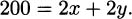
Solving for y, we get
We can use this to eliminate y. If we substitute for y in our area formula, we get
Now we can apply calculus to this function. Taking the derivative, we get
Remember, maxima and minima occur at critical points. There are no places where the derivative is undefined (that is, no places where we do something like divide by zero or take the square root of a negative), so we don’t have to worry about that. That means the only possible critical points happen when the derivative is zero. Solving:
When x = 50, the area is A = x(100 – x) = 50(100 – 50) = 502 = 2500 m2. To verify that this corresponds to the maximum area, compare with the area at values on either side of 50, say 49 and 51.
| x | A(x) |
| 49 | 2499 m2 |
| 50 | 2500 m2 |
| 51 | 2499 m2 |
As we can see, x = 50 m corresponds to a maximum. Since y = 100 – x = 100 – 50 = 50 m, the largest pen that can be made from 200 m of fence is a 50 m × 50 m square.
We always need to check the critical points. It is easy to become lazy, since it is sometimes a fair bit of work to get from the initial statement of a problem, to a function, to the derivative, to the critical points. But it would be a shame to accidently minimize the value of something we intended to maximize simply because we forgot to check!
Other ways to verify that x = 50 m is the location of the maximum pen size would be to realize that A = 100 – x2 is a parabola opening downward (so our critical point marks the vertex of the parabola) or to graph the function on a calculator or computer. The method that we use to check is not so important as remembering to do the checking.
What if you had been challenged to use 200 m of fencing to build a rectangular pen of minimum size? The answer is easy. Use 0 m of the fence to build a 0 m × 0 m pen with a total area of 0 m2.
What if I insisted, as part of the puzzle, that you use the entire 200 m of fence? Derivatives and critical points can’t tell you the answer because we already found that the only critical point happens when x = 50 m, and it corresponds to the maximum area.
Looking at a graph, you might conclude that there is no minimum, since the graph of A(x) is a parabola opening downward. But this is silly, because most of the graph has negative function values, and in the real world the area of a rectangular pen can never be negative. In Figure 4.16 we’ve augmented the graph to emphasize the positive region.
Figure 4.16 The area of a pen cannot be negative.
In mathematical language, this problem is said to be “constrained.” It only makes sense on the closed interval [0,100], and f(x) has two minima on the interval. It has a minimum at each end, at the “boundary” of the interval.
The solutions x = 0 m and x = 100 m make some practical sense, by the way. When x = 0 m, we have y = 100 – x = 100 m. Our rectangle has degenerated into two parallel runs of fence slapped together with no space between then. When x = 100 m, then y = 0 m, and the two strings of fence run the other way. Either solution gives a minimum area for the pen of 0 m2 and uses all of the fence.
You should convince yourself that this does not contradict Observation 1 on p. 254, that a maximum or minimum cannot occur when the derivative of a function is negative. When we made that observation, we depended on there being points to the left where the function would be higher and points to the right where the function would be lower. Obviously, when we come to the end of the interval there are no more points, and a minimum (as we have observed) or a maximum can occur.
In a similar way, a positive derivative will not prevent a maximum or minimum from occurring at the end of an interval. So Observation 2 is not contradicted either.
Optimization principle: For a function defined on a closed interval, maxima and minima may (only) occur at critical points as well as at the endpoints of the interval. We have to check the function at each of these places.
EXAMPLE 4.27A student has 200 m of fence available to make a garden (Figure 4.17). She wants the shape of the garden to be like the free-throw lane on a basketball court, a rectangle capped by a semicircle. What dimensions make the largest garden (or the smallest)?
Figure 4.17 A fenced garden.
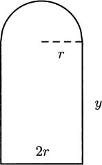
Solution: Deciding how to label a picture can sometimes be a real challenge. For this figure, it probably makes sense to label the radius of the semicircle, since both the area and perimeter formulas for circles are given in terms of r. This forces one side of the rectangle to be 2r, and it is left to label the other side, which we have marked with y in this figure.
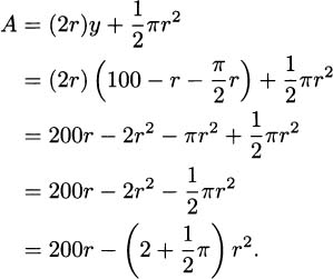
What are we trying to maximize? The area of the garden is the area of the rectangle plus the area of the semicircle, A = (2r)y + πr2. This formula has two variables, so we need to eliminate one before we proceed.
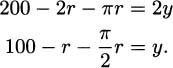
To eliminate a variable, we use the other piece of information that we know, which is that we are to use 200 m of fence. The 200 m perimeter of the garden comes from three sides of the rectangle together with the semicircle:
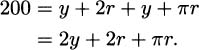
Solve for either r or y by getting it alone on one side:
If we substitute this into the area formula, we get
This is a formula that we can optimize. Before we search for critical points, let’s first determine if there is an interval that constrains the problem. Clearly, r can’t be negative since it represents a real-world distance.
But how large can r become? Since the amount of fence is fixed, as r gets larger it can only be that y becomes smaller. Now, y can’t be negative, so the largest r would correspond to y = 0. To have a perimeter of 200 m, when y = 0 we would need 200 = 2r + πr, and solving,  .
.
So our function is constrained to the interval  .
.
To find critical points, we differentiate:
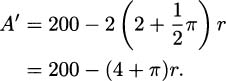
This derivative is never undefined, so critical points can only come from the derivative being zero. Solving:
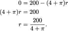
Our optimization principle tells us that to finish, we need to check the function at this critical point and at the ends of the interval.
| r | A(r) |
| 0 | 0 |
| 200/(4 + π) | 2800.5 |
| 200/(2 + π) | 2376.8 |
The smallest garden occurs when r = 0 and y = 100, and it has an area of 0 m2. The largest garden comes from making  , which (if you check) also makes y ≈ 28 m, and it has an area of approximately 2800.5 m2.
4.41 For each function find the critical points and classify each as a maximum, minimum, or neither.
4.42 For each function and interval, find the points where the function reaches its maximum and minimum.
on [2,4]4.43 A rectangular pen runs next to a stream, so one side does not require a fence. Find the dimensions that maximize and minimize the area of the pen assuming 200 m of fence is used.
4.44 A rectangular pen runs along an inside comer of an existing (large rectangular) fence, so two sides do not require a fence. Find the dimensions that maximize and minimize the area of the pen assuming 200 m of fence is used.
4.45 A garden in the shape of the free-throw lane on a basketball court is built with one side against an existing wall, so that side needs no fence as in Figure 4.18. What are the dimensions that maximize the area of the garden?
Figure 4.18 A fenced garden against a wall.
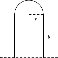
Figure 4.19 A ladder goes around a comer.
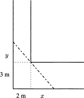
4.46 Imagine carrying a ladder down a hallway when you come to a right-angle comer, as in Figure 4.19. Assume that the ladder is arriving from a hallway that measures 2 m across and entering a hallway that measures 3 m across. If the ladder is too long, it may not make the turn.
4.47 A wire 90 cm long is divided into three straight pieces of wire. Two pieces are the same length, x, which leaves the remaining piece of length 90 – 2x. Use the wire to form an isosceles triangle.
4.48 A string consisting of n 9-volt batteries is connected in series to a 100 ohm circuit. Assume the current supplied (in amps) depends on the number of batteries, n, according to the formula 
We have grown accustomed to prime notation for derivatives; if f(x) is a function then f′(x) is its derivative. This was the notation of Joseph-Louis Lagrange who lived 1736–1813, and it is one of the most popular derivative notations.
Leonhard Euler (1707–1783) used the capital letter D to indicate derivatives. So the derivative of the function f(x) is Df, or Dxf when we want to be explicit about the dependent variable being x.
Isaac Newton, who lived 1642–1727 and was one of the inventors of calculus, used dot notation. If we recall our example of dropping a pen, we had the position formula
To indicate a derivative, Newton placed a dot over the dependent variable, y. In his notation, the derivative (which we now know indicates the velocity) looks like

Gottfried Wilhelm Leibniz, who lived 1646–1716 and is credited along with Newton for the invention of calculus, had yet another notation: differential notation. If y = f(x), then Leibniz’s notation indicates the derivative by the symbol dy/dx.
To understand what Leibniz’s symbol is trying to represent, remember how we came to the idea of derivative. The derivative tells us the slope of a tangent line, and we determine the slope of a tangent line from the slopes of secant lines using a limit.
In normal conversation, we say
But if we take y = f(x), the “rise” is simply the change in y, which we might write as Δy. Similarly, the “run” is the change in x, or Δx. In this context, the slope of a secant line is
The slope of the tangent is defined to be the limit of the slopes of the secants over shorter and shorter intervals, that is, the slope as Δx gets closer and closer to 0:
The Leibniz notation is meant to reflect this process, so
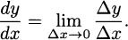
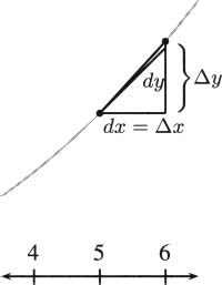
Where we see Δx and Δy we should think of secant lines. A small change in y is divided by a small change in x. Where we see dx and dy, we should infer tangent lines, i.e., the result of taking a limit.
It is common for people to think of dy/dx as an infinitesimal change in y divided by an infinitesimal change in x. Although this is (formally) a lie, since the real number line is usually not considered to contain infinitesimal values other than 0, it is often a useful and tangible way to think of dy/dx.
Derivatives can be useful for estimating small changes in a function. Consider, for example, measuring a square with a ruler. Say we measure the side length to be 5 cm, as in Figure 4.20. Then we know the area to be 25 cm2.
Figure 4.20 Measuring a 5 cm × 5 cm square.
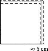
Rulers, however, are not perfect. We never measure a length to be exactly 5 cm. There is always a margin of error. Perhaps we actually know the length to be 5 cm ± 0.1 cm.
Of course, a change in the side length means a corresponding change in the area of the square. We can compute this directly: the largest possible area is 5.1 cm × 5.1 cm = 26.01 cm2, and the smallest is 4.9 cm × 4.9 cm = 24.01 cm2.
We can also estimate this in a calculus context by letting x represent the length of the side we are measuring so that y = f(x) = x2 is the area. Our goal is to estimate the change in f(x) that comes from changing (or mis-measuring) x by a small amount.
We’ve emphasized that the derivative is a limit of slopes of secant lines. Another way of saying this is that when Δx is small, the slope of the secant is approximately the same as the slope of the tangent. When Δx is small,

Multiplying by Δx, we get a formula that estimates the change in the function.
The derivative approximation rule:  .
.
In our case, since y = f(x) = x2, we have dy/dx = 2x. We measured x = 5 cm, but we may have a measurement error as large as Δx = ±0.1 cm. To estimate the error in the area, we compute:
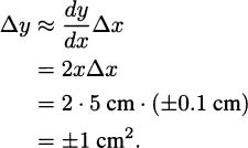
So, we estimate the area of the square to be 25 cm2 ± 1 cm2 ; it may be as low as 24 cm2 or as high as 26 cm2. This estimate matches almost exactly what we obtained by direct computation.
To understand how this estimate works, it may help to look carefully at the graph of f(x) = x2 near the point x = 5.
Figure 4.21 The function f(x) = x2 near x = 5.
In this picture, Δy indicates the true change in the value of a function, the true difference that we could compute by evaluating the function at two points and subtracting. For example, if this is the graph of y = x2 with Δx = 1, then Δy = 36 – 25 = 11.
The value dy is the corresponding change that happens in the tangent line. We know from the derivative that the slope at 5 is f′(5) = 2 · 5 = 10, so the equation of the tangent line (in point-slope form) is y – 25 = 10(x – 5), or in the slope-intercept form, y = 10x – 25. Evaluating at x = 6 and x = 5, we subtract to get dy = 35 – 25 = 10. This is a bit smaller than the true Δy of the function, and we can see this on the graph.
We took Δx = 1 cm, a pretty large change. Imagine how much closer the estimate would be if we took Δx = 0.1 cm. The difference between Δy and dy would be very small. This is the key to approximating with derivatives. For small changes in x, the tangent line is a close approximation to the function, so (vertical) changes measured on the tangent line do a good job of estimating (vertical) changes in the function.
The symbol dy is called the differential of the function. This is why the symbol dy/dx is often referred to as differential notation and why the method of approximating with derivatives is called differential approximation.
EXAMPLE 4.28Estimate  using only the operations available on a 4-function calculator.
Solution: If we let f(x) = , then our task is to estimate the value of f(8.95). Fortunately, the value f(9) = 3 is easy to calculate. We can apply a differential approximation using Δx = –0.05 to see how much f changes as we move to the nearby x-value:
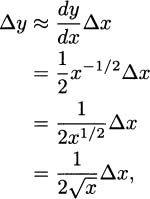
and using x = 9 and Δx = –0.05, we get
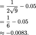
Having estimated the change in function value, we can now calculate that 
 – 0.0083 = 2.9917. We used only addition, subtraction, multiplication, and division (the operations available on a 4-function calculator).
It may have never occurred to you, but even powerful computer chips often know how to do only simple operations. More complicated calculations, such as roots and the values of trigonometric functions, are typically produced by approximation methods programmed in software.
4.49 The side length of a cube is measured to be x = 15 cm with a margin of error of ±0.5 cm. Estimate the change in the volume that results from measurement error.
4.50 The side length of a cube is measured to be x = 15 cm with a margin of error of ±0.5 cm. Estimate the change in the surface area that results from measurement error.
4.51 The radius of a circle is measured to be r = 30 cm with a margin of error of ±1 cm. Estimate the change in area that results from measurement error.
4.52 The radius of a sphere is measured to be r = 30 cm with a margin of error of ±0.1 cm. Estimate the change in volume that results from measurement error.
4.53 The Earth is approximately spherical, with a radius of 6378.1 km. A ‘belt’ of 40074.8 km would wrap around the “waist” of the Earth. If 1 m of slack were added to the belt, how high would the belt rise above the Earth? (Hint: you are given a circumference C with change ΔC, and asked to estimate Δr.)
4.54 The Moon has a ‘waist size’ of 10916.4 km. If 1 m of slack were added to its ‘belt,’ how high would the belt rise above the surface of the Moon?
4.55 Use differential approximation to estimate each value:


 (Hint: 100/49 is a perfect square.)
 (Hint: find a ratio of perfect squares near the value 5.)
If we are a company that manufactures some item, then the marginal cost of the item is said to be the cost of increasing our production level by one item. For example, if we can produce 10 hand-held radios by spending $33.67 for parts and labor, and 11 radios would cost us $35.77, then we can compute the marginal cost to be $35.77 – $33.67 = $2.10. At a production level of 10 radios, the marginal cost for making one more radio is $2.10.
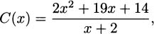
Perhaps for our particular production line, the cost of making x radios is modeled by the function
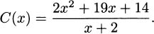
We can make a couple of easy observations. One observation is that the cost of making zero radios is C(0) = 7. In most manufacturing situations there are some expenditures even when nothing is produced. These are called fixed costs. We can also verify the marginal cost for producing the eleventh radio by computing C(11) – C(10) ≈ 35.77 – 33.67 = $2.10.
EXAMPLE 4.29Marginal cost generally depends on the production level, and it is common that the marginal cost decreases as we make more and more items. In fact, you’ve probably heard the phrase “efficiencies of scale.” Verify that the twenty-first item costs less to produce than the eleventh.
Solution: We’ll use the cost function. The cost of the twenty-first item is the difference between the cost for twenty-one items and the cost for twenty items:
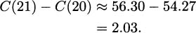
The cost for the twenty-first radio is $2.03, which is less than the $2.10 that the eleventh radio costs to produce.
EXAMPLE 4.30Since the cost function for radios is
the marginal cost function is
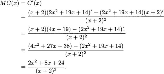
It follows that the marginal cost when producing 10 radios is C′(10) ≈ $2.11, and the marginal cost when producing 20 radios is C′(20) ≈ $2.03.
Notice that we don’t get precisely the same answer when using the derivative as we did by direct computation, but the results are very close. This is because our derivative definition of marginal cost is really a differential approximation of the cost for one more item.
Recall how differential approximation works. For small values of Δx, we know that

or equivalently,
If we take Δx = 1 (we are interested in the change in cost that comes from producing just one more item), we get ΔC ≈ dC/dx. The cost of one more item is approximately the derivative of the cost function. The intuitive definition of marginal cost and the calculus definition are approximations.
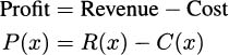
Revenue and profit work the same way.
The marginal revenue is approximately the change in revenue that comes from producing one more item, and the marginal profit is approximately the change in profit from one more item.
This agrees with our intuition. Since profit is revenue minus cost, the profit from one more item should be the revenue for the item after its costs are subtracted.
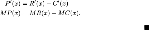
Proof. The rules of derivatives make this easy to verify:
and taking derivatives of both sides,
In a business setting, raising revenues is good. Cutting costs is good. But maximizing profit is best, because that is what puts money in our pockets. If our business is modeled by a cost function and a revenue function, can we determine the production level that maximizes our profit?
Recall from the optimization principle (p. 261) that maxima of a function occur at critical points. We will want to check places where the derivative of P(x) is zero or undefined.
In general we need to worry about derivatives being undefined, but this is not a great worry for the profit function P(x). Remember, the derivative tells us the marginal profit, which is approximately the profit for making one more item. It would be an uncommon scenario where the profit for the next item couldn’t be determined. Consequently, we can assume that critical points of the profit function occur because the derivative is zero.
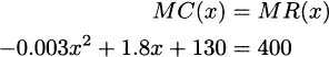
Proof. Maxima (and minima) occur at critical points, i.e., where the derivative is zero or undefined. Since there is not a worry that marginal profit is undefined, maxima (and minima) will occur where the derivative is zero. Calculating:

and, adding MC(x) to both sides, it follows that
We can verify this result intuitively with the following thought experiment. Assume we are manufacturing radios and our current production level is x radios.
If the marginal cost, MC(x), is less than the marginal revenue, MR(x), then we should increase our production level by at least one more radio. It will increase our profit (by increasing our revenue more than our costs). On the other hand, if the marginal cost is more than the revenue, i.e., MC(x) > MR(x), we should produce fewer radios. The cost savings will more than make up for the loss in revenue.
So, the maximum profit can only occur where the marginal cost neither lags nor exceeds the marginal revenue.
A similar argument works for minimum profit. The minimum profit will also occur at a production level where the marginal cost and marginal revenue coincide. If we invoke the precept of Sherlock Holmes yet again, we have to remember that places where the marginal cost and marginal revenue coincide are only “suspects” for the maximum profit. We still have to check each one.
EXAMPLE 4.31Yo-yos sell for $2 each. The cost of producing x yo-yos is C(x) = 50 + 0.01x2.
How many yo-yos should be produced to maximize profit?
Solution: Note that we haven’t been given a revenue function, but we have been given enough information to figure it out for ourselves. Since yo-yos sell for $2, if we sell x of them, our revenue function is R(x) = 2x.
To maximize profit, we want to consider when MC(x) = MR(x), so we compute the derivatives, MC(x) = 0.02x and MR(x) = 2. Setting them equal, we learn that
The profit for 100 yo-yos is R(100) – C(100) = 200 – (50 + 100) = $50. This could be a maximum, but it could also be a minimum (or even just a lucky point where the marginal cost and revenue happened to coincide by accident). We can verify that it is a maximum in several ways, but probably the two most obvious checks are:
We could calculate the profit for 99 yo-yos and for 101 yo-yos and discover that in each case the profit is less than $50 (i.e., less than the profit for 100 yo-yos). It is in fact $49.99 at both x = 99 and x = 101.
We could use a computer or calculator to graph the profit function P(x) = 2x – (50 + 0.01x2), on an interval around 100 and see that x = 100 is the location of the highest point.
EXAMPLE 4.32A plane holds 450 seats. Tickets cost $400 each, and the cost of operating the plane with x passengers is C(x) = –0.001x3 + 0.9x2 + 130x + 3000. How full should the plane be to maximize profit?
Solution: As in the previous example, we have to realize that a $400 ticket price implies that the revenue function is R(x) = 400x. To find critical points of the profit function, we take derivatives and set marginal cost and marginal revenue equal.
Subtracting 400 from both sides gives

Since this is a quadratic equation we can solve with the quadratic formula to get
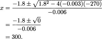
We still need to verify that selling 300 tickets maximizes profit, so we check values on each side:
| x | P(x) |
| 299 | 23999.999 |
| 300 | 24000.000 |
| 301 | 24000.001 |
It looks as though x = 300 is not a maximum. (It is not a minimum either.) Admittedly, the values are very close, so close that we should suspect or at least be cautious about rounding error. Let’s check again, with values a little further from 300:
| x | P(x) |
| 290 | 23999.00 |
| 300 | 24000.00 |
| 310 | 24001.00 |
Indeed, it looks like x = 300 is not a maximum or minimum for profit. That leaves our question unanswered: How many tickets should we sell to maximize profit? The answer is “all of them.”
Here’s how we see that: Since the critical point did not provide an answer, we must look at the boundary, that is, the smallest and largest possible values of x. The fewest number of tickets we can sell is 0, and the most is 450, so this entire problem takes place on the interval [0, 450].
Check the profit at the endpoints of the interval:
| x | P(x) |
| 0 | –3000.00 |
| 450 | 27375.00 |
The profit for selling 450 seats is $27,375.00, which is greater than the value at x = 0 (which generates a loss) and the value at x = 300 where the critical point occurred. A full plane generates the greatest revenue.
4.56 Graph the revenue function R(x) and the cost function C(x) for Example 4.31 together on one graph.
4.57 Graph the revenue function R(x) and the cost function C(x) for Example 4.32 together on one graph.
4.58 At a production level of x = 200 items, MC(x) = 7 while MR(x) = 10.
4.59 I intend to produce computers that sell for $400 each. My cost for producing x computers is C(x) = 1000 + x2/80.
4.60 Assume that the price I can charge for a product drops if I flood the market with items, so that the price I can charge is p(x) = 2000/x.
Since derivatives tell us rates of change, it should be little surprise that calculus is important for the study of different kinds of growth. For example, linear growth (which describes something whose size looks like a line when you graph it over time) is very easy to describe with calculus. Its derivative is a constant (the slope of the line).
One of the most important kinds of growth is exponential growth. It describes many biology situations, such as the growth of a bacteria colony or the spread of a disease. It has a role in computing physical properties such as the decay of radioactive elements, or changes in temperature. It also has applications to finance.
If you invest a sum, say $1000, and you receive simple interest at a rate of 5%, then each year you are paid 5% of your $1000 as interest. Over time, your investment will grow as in the following table:
| years | balance |
| 0 | 1000 |
| 1 | 1000 + 50 |
| 2 | 1000 + 50 + 50 |
| 3 | 1000 + 50·3 |
| 4 | 1000 + 50·4 |
| . | . |
| . | . |
| . | . |
| t | 1000 + 50t |
No matter how many years you maintain your investment, the principal will always be $1000, and the interest payment will be 5% of that $1000. This kind of arrangement is typical for a bond that makes regular payments to you.
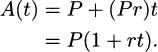
If we write r for the fractional interest rate (i.e., r = 0.05 denotes a 5% rate), and P for the principal invested, then over time the investment is worth
With an investment that pays compound interest, each interest payment is added to the principal. If you invest $1000, earning 5% annually, your principal becomes $1050 after the first year. Consequently the second year’s interest payment will be larger, because it will be calculated based on both the original $1000 investment and the previously awarded interest—5% of the entire $1050. Over time, your compounded investment will grow like:
| years | balance |
| 0 | 1000 |
| 1 | 1000 + 50 |
| 2 | 1050 + 52.50 |
| 3 | 1102.50 + 55.13 |
| 4 | 1157.63 + 57.88 |
| . | . |
| . | . |
| . | . |
| t | ? |
Determining a formula for your investment after t years is a little harder than for simple interest, but not too bad if you write things down the right way. After 1 year, your balance is
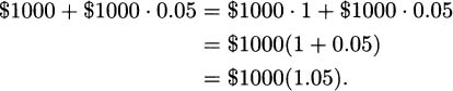
In the second year another interest payment is added, 5% of the new amount, increasing your balance to
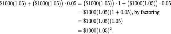
Each year, the new balance is derived from the previous balance by multiplying by 1.05, and the amount after t years is
Again, let r denote the fractional interest rate. If P is the original principal invested and t is years, then the amount the investment is worth after t years (compounded every year) is
Since compound interest is a kind of exponential growth, we take a moment and review some of what we learned from algebra class about exponential functions and their inverse functions, logarithms.
EXAMPLE 4.33The function f(t) = 1.05t is an exponential growth function. The function g(t) = 0.95t is an exponential decay function. Some sample values of each are computed in the following tables.
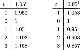
The exponent of an exponential can be any real number, though if it is not an integer we will usually use a calculator or a computer to aid with the calculation. On scientific calculators, the button for computing general exponentials is usually marked with a caret ^ or the expression yx, and it can compute values such as 1.053.3 = 1.17469 and 0.9510.4 = 0.58658 (these are approximate values).
You may also recall from algebra class that we have identity laws for exponentials. We summarize some here:
| axbx = (ab)x | multiplying with same exponent |
| axay = ax+y | multiplying with same base |
 |
dividing with same exponent |
 |
dividing with same base |
 |
reciprocals |
| (ax)y = axy | power of a power |
 |
roots are fractional exponents |
We can readily verify these with a calculator. For example, if a = 1.3, b = 5.5, and x = 3, then

while

We get the same answer either way.
There is one special base that is so important that we reserve a letter for it, and that is the number e = 2.71828182845904523536…. Like π, e has a nonterminating, nonrepeating decimal expansion. Scientific calculators have a key that is usually marked either exp or with the expression ex which calculates exponentials with base e. With your calculator, you can verify a few values of this function.
| t | et |
| –1 | 0.3679 |
| 0 | 1 |
| 1 | 2.7183 |
| 1.5 | 4.4817 |
| 2 | 7.3891 |
Figure 4.22 The natural exponential function f(x) = ex.
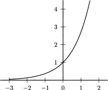
If you inspect the graph of the exponential function in Figure 4.22, you will see that it passes a horizontal line test (horizontal lines intersect the graph in a single point). You may remember from algebra class that functions that pass the horizontal line test have inverse functions. The inverse of the exponential with base a is called the logarithm with base a, and it is sometimes written as g(x) = loga x.
Inverse functions “undo” each other, just as f(x) = and g(x) = x2 undo each other. For example, start with x = 9. Then f(9) =  = 3, and the reverse process that takes us from 3 back to 9 is g(3) = 32 = 9.
For the calculus student, the most important logarithm function is the logarithm with base e, which is called the natural logarithm, since it is the inverse to the natural exponential function. The notation for the natural logarithm is g(x) = ln x. Scientific calculators have a key labeled ln that computes natural logarithms, not to be confused with the log key which computes common (base 10) logarithms.
Using a calculator, we can verify the inverse relationship of the natural exponential and natural logarithm functions. First, compute e1.5 = 4.4817. Then check that ln(4.4817) = 1.5. It works the other way too, that is, computing the logarithm first and then doing the exponential. For example, compute that ln(10) = 2.3026 and verify that e2.3026 = 10.0.
Figure 4.23 The natural logarithm function f(x) = ln x.
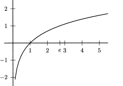
Some values of the natural logarithm are given in the table below. You may wish to check that you can produce them with your calculator. Notice that they agree with the graph of the natural logarithm in Figure 4.23.
| t | ln(t) |
| 0.5 | –0.6931 |
| 1 | 0 |
| 1.5 | 0.4055 |
| 2.0 | 0.6931 |
| e | 1 |
| 5.0 | 1.6094 |
Some computer programs use log(x) to denote the natural logarithm. If you suspect this, you can check by computing log(10). If you get an answer of 2.302585, then it is the natural logarithm. The common logarithm would return 1.0.
As with exponentials, there are identity laws for logarithms that help us with computations. Versions of these work with logarithms of any base, but we focus on the natural logarithm.
| ln(et) = t | property of inverses |
| eln t = t | property of inverses |
| ln (ab) = ln(a) + ln (b) | log of a product |
 |
log of a quotient |
| ln (at) = t ln(a) | log of a power |
 |
change of base rule |
EXAMPLE 4.34If I invest $1000 and receive 5% interest compounded annually, how long will it be before I have $5000?
Solution: We computed previously that the amount of money after t years is
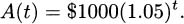
We need to find the value of t when A(t) = $5000. Solving,
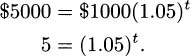
Here, we can take the logarithm of both sides.
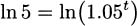
Apply the identity for log of a power to the right-hand side.
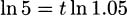
Now get t alone on one side.
It takes about 33 years for this $1000 to grow to $5000.
We saw that $1000 invested at a simple interest rate of 5% has a value over time of A(t) = P(1 + rt) = 1000(1 + .05t) = 1000 + 50t. What happens if we take the derivative of this function?
The answer is A′(t) = 50. Does this represent anything useful? It does indeed, and recalling the differential notation can make it a bit more apparent. We could just as correctly have written,

The derivative tells us the (instantaneous) rate of change of the amount over the time. Consider the units that apply here. A change in A, which we write as ΔA is measured in dollars. A change in t is measured in years. The fraction dA/dt is the (instantaneous) slope of the function, measured in dollars/year. It tells us how fast our money is growing at any moment, at a rate of 50 dollars/year.
We don’t yet have a formula for the derivative of an exponential function, such as A(t) = 1000(1.05)t. It is tempting to try to apply the power rule, but that is a mistake. A power, like x2, is not an exponential, like 2x. A different rule applies.
It turns out that the slope of an exponential function is always proportional to the height of the function at the point of tangency (i.e., there is some constant number that you multiply the value of the function by to get the slope). We get a sense of this if we remember that
If we take Δt = 1, then ΔA is the amount an investment will grow over the period of 1 year, and that amount is the interest rate times the current amount. If A(t) = 2000 for some t and r = 0.05, then we know that
This is an approximation of the slope, but for the derivative we want the exact slope. To discover this, we’ll take a detour and look at the natural exponential function, ex.
You may wonder what is so ‘natural’ about the natural exponential function. It is natural because it has a simple differentiation formula.
The natural exponential rule: The derivative of f(x) = ex is f′(x) = ex. The natural exponential function is its own derivative.
Figure 4.24 The natural exponential function is its own derivative.
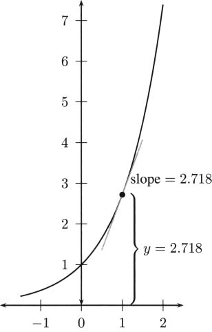
At any point on the graph of y = ex, you’ll find the slope of the tangent line is the same as the height of the graph. Check, for example, by sketching a tangent at the point (0,1), and notice that your line has slope 1 (it extends up at a 45 degree angle). In Figure 4.24 the tangent at the point (1, e) has slope e, as we expect.
The natural exponential is the only exponential equal to its derivative. The derivative of any other exponential function contains an extra constant.
The general exponential rule: If a > 0 is any real number, then the derivative of f(x) = ax is f′(x) = ax ln a.
EXAMPLE 4.35Find the derivative of A(t) = 1000(1.05)t.
Solution: By the general exponential rule,
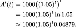
As promised, the derivative is proportional to the function A(t). That is,
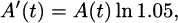
and the constant of proportionality is ln 1.05 ≈ 0.04879. Also note that 0.04879 is approximately the same as the interest rate of 0.05. Of course, 0.05 appears in the derivative estimate we would get from using Δt = 1, i.e., if we computed A′(t) ≈ A(t + 1) – A(t) = 1000(1.05)t+1 – 1000(1.05)t = 1000(1.05)t(0.05).
EXAMPLE 4.36What is the slope of the tangent to A(t) = 2000(1.07)t, when t = 0? What about when t = 3?
Solution: The derivative of A is A′(t) = 1000(1.07)t ln 1.07, so the slope when t = 0 is A′(0) = 1000(1.07)0 ln 1.07 = 1000 ln 1.07 ≈ 67.66. The slope when t = 3 is A′(3) = 1000(1.07)3 ln 1.07 ≈ 82.88.
Like the natural exponential function, the natural logarithm function has a nice derivative.
The natural logarithm rule: The derivative of f(x) = ln x is f′(x) = 1/x.
Figure 4.25 shows a graph of y = ln x together with a tangent line at x = 2. Notice that the slope appears to be 1/2, as the natural logarithm rule states. Ask yourself, what should the slope be when x = 1? Does the graph look right to you at that point?
The natural logarithm rule “fills in” a hole that we had in our differentiation rules. For each power, f(x) = xn there is a function that we can take the derivative of to get f, except in the case where n = – 1. For example,  , and
, and  . In general,
  , as long as n ≠ –1. So, until we learned the derivative of the logarithm, we did not have a function whose derivative was x–1 = 1/x.
Figure 4.25 The derivative of ln x is 1/x.
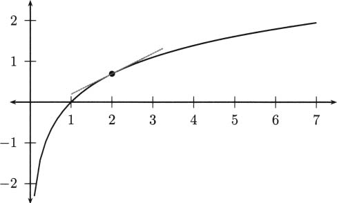 EXAMPLE 4.37
The number of computer clock cycles a particular computer program needs to sort n items of data is given by the formula T(n) = 7000 + 1440n ln(n). For example, sorting n = 2000 data items requires about T(2000) ≈ 21.9 million clock cycles. At what rate is the sort time changing when n = 2000?
Solution: Since we are asked for a rate, we know that the answer is a derivative. It is reasonable to ask “what is the variable?” and “what is the function?” In this case, the variable is n, the number of items we wish to sort. The function is T, the time required to sort n items.
The rate we want is then the change in T with respect to n, or  . Using the sum and constant coefficient rules we have
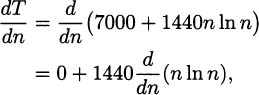
and applying the product rule and natural logarithm rule yields
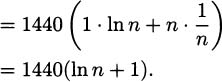
If we evaluate at n = 2000 we get 1440(8.6) ≈ 12,385 cycles/item. The computer program requires approximately 12,385 cycles to accommodate another sort item.
To check, let’s compute directly the difference between sorting n = 2001 items and n = 2000 items (without calculus).
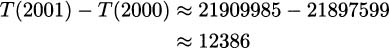
This agrees well with our derivative calculation. ?
4.61 If I invest $ 1500 and receive a return of 6% simple interest for two years, how much money will I have?
4.62 If I invest $5000 and receive a return of 8% simple interest,
4.63 If I invest $5000 and receive a return of 8% compounded annually, how many years will it take to grow to $50,000?
4.64 The “rule of 72” says that if you receive a compound annual interest rate of p%, then the number of years it takes for your money to double is 72/p years. So, a 6% return will double your money in approximately 72/6 = 12 years.
4.65 Every exponential function f(t) = A · bt can be rewritten using the natural exponential function in the form f(t) = Pert. Find suitable P and r so that 1000(1.05)t = Pert by applying these steps:
4.66 If we invest $1000 at a 6% interest rate compounded monthly, then the balance after t years is  . Find suitable P and r so that 1000(1.005)12t = Pert.
4.67 Compute the derivative of each function.

4.68 Find the equation for the tangent line to y = ex at the value x = 1, as illustrated in Figure 4.24.
4.69 Find the equation for the tangent line to y = ln x at the value x = 2, as in Figure 4.25.
4.70 During the Cold War, nuclear detonators were made from radioactive Polonium-210. Because it is highly radioactive, Polonium-210 quickly decays into other elements. If a detonator initially contains 11 mg of Polonium-210, then the amount (in mg) remaining after t days is A(t) = 11e–0.00502t.
Think about riding a Ferris wheel. What are the aspects of the ride that make it enjoyable? As you turn about the wheel, you initially rise up the back side, and the lift of the wheel presses you down into the seat. There’s the moment where you “hang” at the top, and then you fall down the front side.
The sensations of a Ferris wheel come predominantly from the interaction of gravity with the centrepital (due to rotation) force you experience, but you might wonder related questions like “how fast am I falling (vertically) when I go around the wheel?” When is the vertical acceleration the greatest? When is it the least?
You may recall from trigonometry that, on a circle of radius r, a point (x, y) is completely determined by the angle θ of a ray from the origin, as in Figure 4.26.
Figure 4.26 The circular functions y = r sin θ and x = r cos θ.
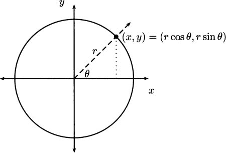
The ratio of y to r is given by the sine function,

Another way to say this is that if you know θ and r, then the y coordinate must be y = r sin θ. Similarly, the cosine function relates the x coordinate to the radius:

Equivalently, x = r cos θ.
If we are to use sine and cosine with our calculus, we’re going to need to know the derivative of each. Although these differentiation formulas can be proven, here we will guess the formulas from graphs.
Note, in calculus we almost always take angles to be measured in radians (that is, a complete circle is 2π radians rather than 360°). Just as you measure temperature in Celsius (or when things really matter, in Kelvin) when doing chemistry, if you want your mathematics to turn out right in calculus class, your best bet is to work in radians.
Look carefully at the sine function in the top graph of Figure 4.27. A small piece of tangent line has been added at each of the multiples of  . Notice at
  , for example, that the slope of the tangent is 0. At the origin, the tangent line appears to have slope 1. Now compare with the points added to the bottom (cosine) graph. The slope of each tangent to sine has been plotted on the cosine graph.
When the slope of sine is zero, the cosine graph has value zero. When the slope of sine is 1, the cosine has value 1. In each case, the slope of the sine curve is precisely the value on the cosine curve. Thus, the cosine function tells the slope of the sine function. That means that the derivative of y = sin t is the function y = cos t.
Figure 4.27 Graphs of y = sin t and y = cos t.
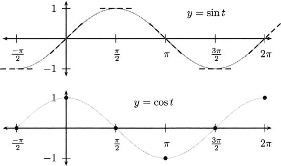
The sine rule: The derivative of f(x) = sin x is f′(x) = cos x.
EXAMPLE 4.38What is the tangent line to y = sin x when x = π/6?
Solution: For a tangent line, we need a point and a slope. The y coordinate of the point of tangency is y = sin(π/6) = 1/2. The slope is given by the derivative, m = cos(π/6) =  . Using the point-slope form of a line, the tangent is
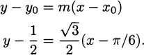
In slope-intercept form, this is

There are several ways to determine the derivative of cosine, and perhaps the most obvious is to do what we did for sine, draw a graph and guess. But we can also derive the rule for cosine from the existing sine rule, because sine and cosine are related by a cofunction identity. For any angle θ, the complementary angle is 90° – θ, and cos θ = sin(90° – θ). Figure 4.28 illustrates this relationship on a triangle.
Figure 4.28 Complementary angles: cos θ = sin(90° θ) = x/r.
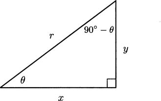
If we know the complementary angle formula, we can derive a derivative formula for cosine. First we switch to radians, and then we differentiate using the chain rule:
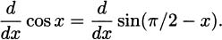
On the right hand side, the outside function is g(x) = sin x and the inside function is f(x) = π/2 – x. By the chain rule,
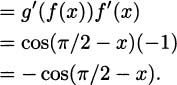
There is one last trick, and that is to use a cofunction identity again to replace cos(π/2 – x) with sin x,

The cosine rule: The derivative of f(x) = cos x is f′(x) = – sin x.
EXAMPLE 4.39What is the derivative of y = x2 cos(3x + 1)?
Solution: All of our usual rules (product rule, chain rule, etc.) apply to trig functions. So, beginning with the product rule,

and continuing with the chain rule,
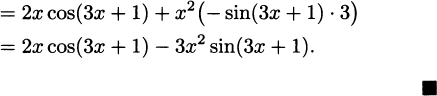
We now have the tools we need to answer questions about Ferris wheels. The Beijing Great Wheel, planned to be the tallest Ferris wheel in the world if completed, will have a wheel of diameter 99 m and reach a total height of 208 m. One revolution of the wheel requires 20 min (1200 s).
A function that models the height of a point on this wheel, with t given in seconds, is
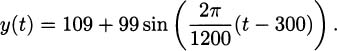
To verify this, check that t = 0 gives a height of 10 m (the lowest the wheel achieves):
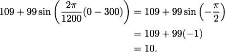
After 10 min (600 s), the function reaches its maximum height,
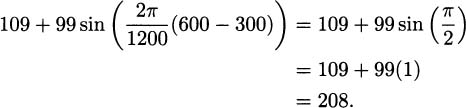
EXAMPLE 4.40What is the vertical velocity of a point moving around the Great Wheel at time t = 0,150, 300, or 600 s?
Solution: We need to compute the derivative.
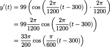
This yields vertical velocity values (in units of m/s) of
| t | y′(t) |
| 0 | 0 |
| 150 | 0.3665 |
| 300 | 0.5134 |
| 600 | 0 |
4.71 Find the derivative of each function.

4.72 In Figure 4.29 the top function is y = cos t, and the bottom function is y = sin t. Where each piece of tangent line occurs on the top graph, draw a corresponding point on the bottom graph representing the slope. Use these values to guess the derivative of cosine.
Figure 4.29 Graphs of y = cos t and y = sin t.
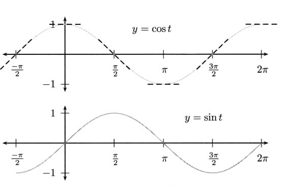
4.73 Write  and use the quotient rule to find a derivative formula for the tangent function.
4.74 Write  and differentiate to find a derivative formula for the secant function.
4.75 Write  and differentiate to find a derivative formula for the cosecant function.
4.76 Write  and differentiate to find a derivative formula for the cotangent function.
4.77 From trigonometry, we know the identity sin 2t = 2 sin t cos t.
4.78 The horizontal position of a point on the Beijing Great Wheel is modeled by the function
Although computing areas may seem like an abstract geometrical task, the (calculus) techniques for finding general areas are also used to solve physical problems such as finding the height of a rock thrown into the air or even a rocket accelerating into space. The same techniques can be used to compute physical work, such as the work required to lift an elevator and its cabling to the top of a shaft or the work required to pump the water out of a swimming pool.
If you consider the kinds of shapes you already know how to find the area of, you may find that the list is pretty short. Most of us know that the area of a parallelogram (and consequently a rectangle and a square) is base × height, and the area of a triangle is × base × height (because two triangles together make a parallelogram). We can compute the area of any shape made from straight sides by cutting it into triangles.
Can you compute the area of any curved shapes? Many people know that the area of a circle with radius r is A = πr2. Unless you’ve been a student of calculus, that’s probably the extent of your knowledge of curved areas.
We would like to be able to find areas of many curved regions. For instance, what is the area under the function y = x2 as x goes from 0 to 1? This is the shaded area in Figure 4.30.
We can see right away that whatever the area under the curve is, it must be less than 1, since the shaded region fits entirely inside a 1 × 1 square. In fact, it fits entirely inside a triangle with vertices at (0,0), (1,0), and (1,1), so the area must be less than 1/2.
Can we say what the area must be bigger than? A rectangle with vertices (0.5, 0), (0.5, 0.25), (1, 0.25), and (1, 0) fits entirely within the shaded region, and the rectangle has area 1/8, so we know the area must be larger than that.
There is a standard (clever) way to estimate unknown areas using shapes that are easy to understand, and it works much like the exploring we are doing here. You find easy-to-compute areas that contain your region and you find easy-to-compute areas contained entirely inside your region. The answer you desire must be somewhere in between. We always make our easy-to-compute areas from rectangles.
Figure 4.30 The area under x2
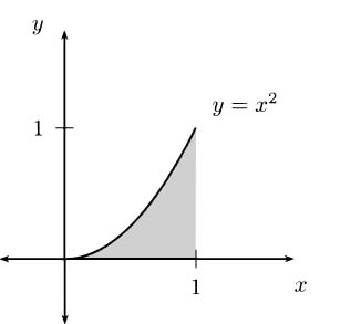
For example, divide the interval [0,1] into five congruent subintervals, at the values x0 = 0, x1 = 0.2, x2 = 0.4, x3 = 0.6, x4 = 0.8, and x5 = 1.0. In each little interval, find the largest value of the function f(x) = x2. For example, on the interval [0,0.2] the highest value of the function is f(0.2) = 0.22 = 0.04. Use that highest value to create a rectangle, as in Figure 4.31.
Figure 4.31 Rectangles that fit over the function y = x2.
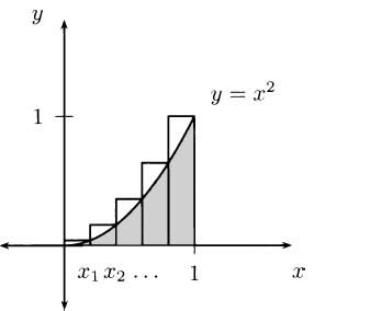
We can tabulate an (over-)estimate for the shaded area:
| width | height | area |
| 0.20 | 0.04 | 0.008 |
| 0.20 | 0.16 | 0.032 |
| 0.20 | 0.36 | 0.072 |
| 0.20 | 0.64 | 0.128 |
| 0.20 | 1.00 | 0.200 |
| total area | 0.440 | |
A collection of rectangular areas, summed to estimate the area of a curved region, is called a Riemann sum, after the German mathematician Bernhard Riemann (1826–1866). Riemann is famous, not only for his work on calculus, but for work in number theory (where the Riemann hypothesis is well known) and for foundational work in the mathematical branch now known as Riemannian geometry.
Notice that this Riemann sum comes to a bit less than 0.5, which was our first over-estimate for the shaded area. You can probably imagine what would happen if we were to use more rectangles. With 10 rectangles, we get an estimate for the area of 0.385 (check for yourself; the calculation is not difficult). As we use more and more “upper” rectangles, the estimates will continue getting lower and lower, becoming closer and closer to the area we are interested in.
Figure 4.32 Rectangles that fit under the function y = x2.
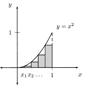
We can do something similar with rectangles lying under the curve, as in Figure 4.32. For example, in the subinterval [0,0.2], the smallest value of the function y = x2 is 0. The only rectangle that could fit “under” the curve is a flat line, with no area at all. On [0.2,0.4] the smallest value of the function is 0.22 = 0.04. As before, we can tabulate an estimate of these “lower” rectangles:
| width | height | area |
| 0.20 | 0.00 | 0.000 |
| 0.20 | 0.04 | 0.008 |
| 0.20 | 0.16 | 0.032 |
| 0.20 | 0.36 | 0.072 |
| 0.20 | 0.64 | 0.128 |
| total area | 0.240 | |
As we did with upper rectangles, we can use more and more lower rectangles to get better (under-)estimates for the area. For example, 10 rectangles yields an area estimate of 0.285 (check for yourself).
Although we can get as close as we like, no finite number of upper or lower rectangles will exactly measure the area we want. Fortunately, there is a deep connection between derivatives and areas.
EXAMPLE 4.41What is the area below the function f(x) = x2 on the interval [0,1]?
Solution: The Fundamental Theorem of Calculus tells us that to compute this area exactly, we only need to find some function F(x) whose derivative is x2. The function  works. Once we find F, we evaluate it at the ends of the interval and subtract, so the area is F(1) –
  .
.
Notice that 1 /3 is between the lower and upper estimates that we computed earlier using lower and upper rectangles.
EXAMPLE 4.42What is the area below the function  on the interval [0,2]? See Figure 4.33.
Figure 4.33 Area under  from 0 to 2.
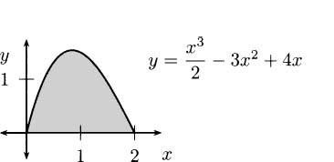
Solution: We need a function  . If we take F(x) =
  – x3 + 2x2, that works exactly. By the Fundamental Theorem, the area is F(2) F(0) = 2 – 0 = 2.
4.79 Estimate the area under the function f(x) = x2 on the interval [0,1] using ten equal subintervals and computing the Riemann sum using upper rectangles.
4.80 Estimate the area under the function f(x) = x2 on the interval [0,1] using ten equal subintervals and computing the Riemann sum using lower rectangles.
4.81 The function F(x) =  + 7 has the property that F′(x) = x2. Use this fact to find the area under the function f(x) = x2 for 0 ≤ x ≤ 1.
4.82 Let f(x) = x – 2.
4.83 For each function f(x), find a function F(x) with F′(x) = f(x).

Area is an important mathematical concept, and like other mathematical notions it has its own notation and careful definition. Informally, you can take the symbols
as representing the area under the function y = f(x) between the values of a and b. In words we read this aloud as “the integral from a to b of f of x dee-ecks.”
We call such an integral a definite integral, since it is defined on an actual (definite) interval [a, b]. The numbers a and b are called the lower limit and upper limit of the integral, respectively. Computing this area is “finding” or “taking the integral of f.” The process of finding an integral is called integration.
In the last section, we took for granted that we could find the area under a curve such as y = x2 or y = sin x and then started looking at rectangles. But mathematicians are typically too careful to assume an answer will exist because it looks good in a picture. Mathematical objects can be surprisingly subtle. (For example, there is an object that has a finite volume and an infinite surface area. If you are curious, you may want to research Gabriel’s Horn or Torricelli’s trumpet.)
So, while we started with the intuitive idea of area and explored it by looking at rectangles, it turns out that mathematically that it should work the other way around. Mathematically, there is no question that any interval [a, b] can be divided into subintervals. Any function defined on an interval [a, b] can be evaluated at points of our choosing (including in each subinterval). So we can always form rectangles that match the height of a function in subintervals of [a, b].
Figure 4.34 An area estimated by general rectangles.
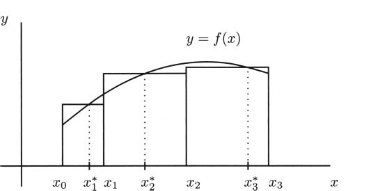
While we can’t guarantee that our intuitive idea of area is correct, the process of taking rectangle estimates is completely rigorous. So this is actually how we define integrals (and we intuitively understand them to be areas). The definition of the Riemann integral is a limit of a sum of rectangles.
We have a lot of freedom about how we choose our rectangles. For example, it is convenient for all the rectangles to have the same width, but that is not necessary. In Figure 4.34 we can see an estimate made with three non-uniform rectangles.
The points that set the heights of the rectangles can be the left endpoint of each subinterval, or the right endpoint, or the midpoint. In fact, when you use more and more rectangles (when you take a limit), it doesn’t matter what point in each subinterval you use to set the height of the rectangle. We don’t even have to choose the same way in every interval, we just need some point in each interval. It has become convention to use “star” notation to indicate this. The value  can be anywhere in [x0, x1]. In general,
  can be anywhere in the zth interval, [xi–1, xi].
In Figure 4.34 the height of the function at would be written f(), so the area of the first rectangle is height × width = f()(x1 – x0). The areas of the other rectangles are computed similarly, so the entire area estimate with all three rectangles would be

As we use more and more rectangles, the sums become tedious to write, so we usually use some abbreviation. We write Δxi for the quantity xi – xi–1, which is the width of the ith subinterval. This makes our sum simpler:
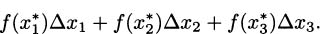
In general, an area estimate with n rectangles looks like

Finally, as we use more (progressively narrow) rectangles, the area estimates often approach a single value. Another way to say this is that the sums have a limit as n (the number of rectangles) approaches infinity. Mathematically, we use this limit to define the integral:

In plain English, a Riemann integral is defined to be the limit of sums of (very narrow) rectangles. If the sums converge to some answer, then we define that to be the integral and refer to it as the area under the curve.
When you understand that the integral is defined in terms of sums, the notation for an integral makes more sense. It is an elongated ‘S’, standing for “sum.” Gottfried Wilhelm Leibniz (1646–1716) introduced the concept of the integral, and the notation, but it was Bernhard Riemann (1826–1866) who defined the integral formally and rigorously.
With this new notation, we can restate the major theorem we use to compute integrals, the Fundamental Theorem of Calculus, expounded by Barrow, Leibniz, and Newton:
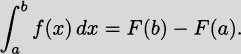
The function F(x) in the Fundamental Theorem is called an antiderivative of f(x). We say “an” antiderivative instead of “the” antiderivative, because antiderivatives are not unique. For example, F(x) = x2 and F(x) = x2 + 14 are both antiderivatives of f(x) = 2x.
The more antiderivatives we are able to compute, the more integrals we can find. That makes antiderivatives and antiderivative formulas important to us. It also means that we’ll want a notation for antiderivatives.
 dx represents an antiderivative of f. It is also referred to as the indefinite integral of f.
Even though we say “the” indefinite integral, we must remember that a function has many antiderivatives. Sometimes we refer to the general antiderivative by giving a formula for all of these antiderivatives at once. For example, the general antiderivative of f(x) = 2x is F(x) = x2 + C, where we understand C to be any constant.
Many of the derivative rules that we studied in Sections 4.5–4.7 have corresponding antiderivative (integral) rules.
The power rule: If n ≠ – 1, then
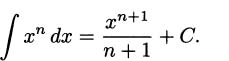
For example,  x6 dx = x7/7 + C.
There are also an integral sum rule and a constant coefficient rule.
The sum rule: The integral of a sum is the sum of the integrals:
The constant coefficient rule: If c is a constant, then
EXAMPLE 4.43Find the general antiderivative of the polynomial f(x) = 12x3 – 5x2 + 1.
Solution: If we carefully apply the preceding rules, we get
In the last line of our calculation, we recognize that C1, C2, and C3 are all constants, and a sum of different constants (even when scaled by multiplying or dividing by some fixed number) is merely another constant.
We can easily check that we are correct. If we take the derivative of our answer, we get f(x) back.
4.84 Find each indefinite integral (general antiderivative).
4.85 Find each area
You might wonder what an integral represents for a function that takes both positive and negative values. For example, we can use the Fundamental Theorem of Calculus to compute
Figure 4.35 illustrates this situation.
Figure 4.35 Signed area under  from 0 to 4.
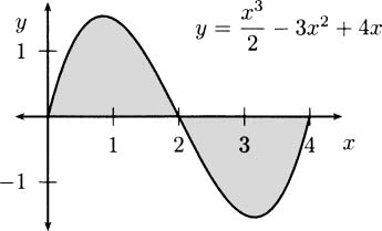
The integral is zero because the area under the curve over the interval [0,2] is counted as positive area, and the area above the function on the interval [2,4] counts as negative area. There are precisely matching amounts of positive and negative area, and they cancel each other out.
We can be sure this is correct if we think about the Riemann definition of integral. Consider dividing the interval [0,4] into small subintervals, and creating a rectangle approximation. The area of the ith rectangle is

If  lands in the left half of the interval, then
  is positive. In the right half of the interval, is negative. The width of a rectangle, Δxi, is always positive.
Since we get a sum of “positive rectangles” from the left half of the interval and “negative rectangles” from the right half of the rectangle, the definition verifies that (when we take the limit) the integral will be the sum of the “signed areas.” In this case, we computed this to be zero, and we can see this is zero in the figure. There is an important principal here.
If a quantity is represented by a limit of Riemann sums, then it is computed by taking an integral.
In geometry, we don’t speak of positive and negative areas. Areas are always positive. But for functions that take positive and negative values, the Riemann sum essentially counts positive areas above the x-axis and negative areas below. So the integral does the same.
Although it is intuitive to think of integrals as (signed) areas, anything that can be represented as the limit of a Riemann sum will be an integral, even if you can’t imagine it as an area.
EXAMPLE 4.44Imagine that you are in a car driving away from town. To keep a record of your speed, you’ve modified your car with a scrolling paper roll (like a seismograph) attached to the speedometer. When you go faster, the “seismograph” pen moves up, and when you go slower, the pen moves down. Perhaps it creates a graph like Figure 4.36.
Figure 4.36 Speed of a car recorded over time.
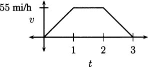
On this trip, the car starts from rest. We can see that, because the curve starts at (0,0). The pen makes a mark on the graph for t = 0 indicating that the speed is y = 0 mi/h. Over the first hour of the trip, the car accelerates evenly until it is traveling 55 mi/h, and it maintains that speed for the next hour before slowing to a stop over the next hour.
Consider dividing the interval into subintervals, and creating the rectangles of a Riemann sum, as in Figure 4.37.
Figure 4.37 Speed of a car recorded over time.
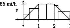
Each rectangle is formed the same way, by taking some reading of the speedometer (measured in mi/h) for the height of the rectangle and a time interval (measured in hours) for the width of the rectangle.
What does the area of a rectangle represent? Looking at units, we can see that the height of the rectangle is mi/h, so the height of the rectangle is a rate. The width of the rectangle is in hours, so it represents an elapsed time. Since distance = rate × time, the area of the rectangle appears to represent a distance.
When the car moves at a constant rate, as it does between t = 1 and t = 2, then the area of a rectangle is exactly how far the car moves in an interval. For example, if the car travels 55 mi/h for 0.5 h, then it covers a distance of 27.5 mi.
When the car is changing speed (either speeding up or slowing down), then we can’t expect things to work out so exactly. But imagine using more and more rectangles, so that the time intervals are very short (and the speedometer doesn’t have time to change much in any interval). If the speedometer shows approximately 40 mi/h for 10 seconds, which is 1/360 of an hour, then a good estimate for the distance traveled would be
If we consider cutting the trip into many 10-second time intervals, we can estimate the total distance traveled by the car as the sum of these rectangular areas. The Riemann sum approximates the length of the trip, and the estimate is better when the intervals are shorter. It seems clear that the true length of the trip is found in the limit: the area under the curve measures the distance the car has moved.
In Section 4.2 we saw that the derivative of position is velocity. In this example we saw that the integral of velocity is (change in) position. This is clear if we think about what the Fundamental Theorem of Calculus (FToC) says.
The FToC tells us that the area over an interval and under a function can be computed by finding an antiderivative and subtracting the values at each end of the interval. Since the velocity of a car is the derivative of the position of the same car, the FToC guarantees that the integral of the velocity is the change in position (the distance the car has moved). In symbols:
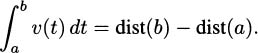
These ideas apply to any rate. If f(t) is the cash flow of a company (in dollars/day), then  is the total change in cash during a 30-day period, i.e., the total net money earned or lost. If E(t) is the energy consumption of the United States (in quadrillion BTU/year), then
  is the total energy consumed in a decade (in quadrillion BTU).

denotes the total change in F between time a and time b.
EXAMPLE 4.45A lead ball is dropped from a tower. How fast is the ball moving after 1.5 seconds?
Solution: To calculate this, we need to know one empirical fact. The acceleration of gravity is (essentially) a constant: –9.8 m/s2. Acceleration is the rate of change in velocity, so integrating the acceleration function tells us the total change in velocity of the ball:
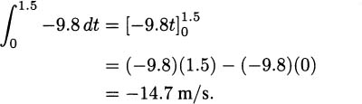
Since the ball was dropped, it started at 0 m/s. The velocity changed by –14.7 m/s as it fell, so the final velocity after 1.5 s is –14.7 m/s. The negative answer indicates that the ball is falling (its height is decreasing). ?
EXAMPLE 4.46A lead ball is thrown upward at 5 m/s from the top of a tower and then falls. How fast is the ball moving after 1.5 seconds?
Solution: In this example the acceleration of gravity is still – 9.8 m/s2, and the total change in velocity is still the same integral with the same result, –14.7 m/s. However, since the ball started with a velocity of 5 m/s, the final velocity is 5 m/s –14.7 m/s = –9.7 m/s.
4.86 A math professor is pushed from the top of a 30 m building.
4.87 A math professor launched from a cannon has a velocity function of v(t) = 9 – 9.8t m/s, where t is measured in seconds from the time the cannon fires.
4.88 The rate of fossil fuel consumption in the United States (in quadrillions of British thermal units per year) is approximately  , where t is years since 1900. How much fuel was used between January 1, 1900 and January 1, 1910?
4.89 A yo-yo company has a profit rate of $20,000 per day when a new advertising campaign begins. Profits rise $1,000 per day, each day, for the next six weeks.
If we know some simple facts, we can estimate some pretty cool things using only basic calculus. For example, we can figure out roughly how high the Space Shuttle flies, knowing only a few facts about the Shuttle. Calculus really is rocket science.
Although the space shuttle no longer flies, when it did, the first part of the ascent was accelerated by the three main engines as well as two solid rocket boosters (which then detached and fell in the ocean).
In the previous section, we learned that integrating an acceleration function will give us the total change in velocity of an object. In the same way, integrating a velocity function gives us the total change in position of an object. So, if we can determine the acceleration function of the Space Shuttle, then determining the height should be a matter of integrating two times, once to get the velocity and again to get the height.
The facts we need to know about the Shuttle are:
Newton’s second law of motion tells us that force is mass times acceleration, or symbolically,

We are interested in the acceleration generated by the rocket engines, so we solve and substitute the facts that we know:
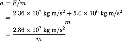
If we knew the mass of the Shuttle, then this calculation would be complete. You may be thinking that we already know that the mass of the Shuttle is 2.0 × 10⁶ kg, but that is not quite correct. The mass certainly starts at two million kilograms, but only two minutes later more than half of the mass has been expended in the form of 1.18 million kilograms of burned fuel. That average rate of fuel use amounts to
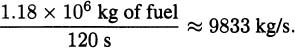
So the mass of the Shuttle is a function of time. We don’t know that the Shuttle uses fuel at a constant rate, but that’s probably not a bad guess. That means that after t seconds, the mass in kilograms is m(t) = 2.0 × 10⁶ – 9833t kg. Using this in the acceleration equation, the acceleration due to the engines is
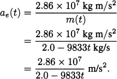
Of course, the engines are not the only acceleration that a rocket experiences. Gravity is also pulling it toward Earth. Fortunately, even for rockets enduring a launch, the acceleration of gravity is easy to compute. It is effectively constant, with the well-known value —9.8 m/s2. Combining this with the acceleration due to the engines, we get the total acceleration on the rocket (as a function of time):
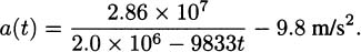
We should be able to integrate this to get the velocity and height of the rocket.
We know that the velocity of the rocket, v(t), will be an antiderivative of a(t), so we integrate:
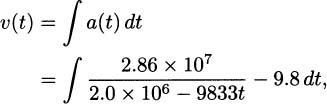
which by the rules of integrals is
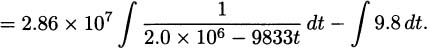
An antiderivative for the second integral is easy to find, since it is the integral of a constant, so let’s focus on the first integral. It is a bit trickier, but not extremely hard.
Let  . Then by the chain rule,
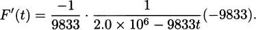
So F is an antiderivative that we can use to compute the integral. Thus
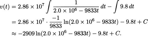
To find the value of C, remember that v(0) = 0 since the rocket starts resting on the launch pad. That means

and solving, we get C = 2909 1n(2.0 × 10⁶) ≈ 42206. So, our velocity function must be

To find the velocity after 2 minutes, for example, we compute

In miles per hour, this is

We’re only one step away from deriving the height of the rocket. In the last step, we computed that the velocity function of the rocket is

Since velocity is the derivative of position (the height) we need only integrate one more time. You may quiver at the thought of finding an antiderivative for v(t), but at least some parts of it are easy. The last term is simple:
And the lines term is too:
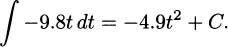
The remaining term is going to take a little more work, but the rules of integrals at least let us factor out the constant in front:

At its heart, the expression we need to integrate is a logarithm. Alas, we haven’t learned an antiderivative for In t. But this doesn’t mean that no one has, and if you were to consult a table of integrals or use a computer program, you would find that t(In t – 1) is an antiderivative for In t.
We know how to take derivatives, so nothing stops us from checking this for ourselves. Let F(t) = t(ln t – 1). Then by the product rule,
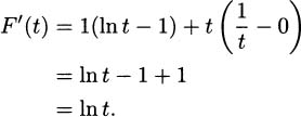
So, we know an antiderivative for In t. Can we build that up to an antiderivative for the expression we need to integrate, namely, ln(2.0 × 10⁶ – 9833t)? If we start from F(t), our antiderivative for In t, we might think to try F(2.0 × 10⁶ – 9833t), and that’s a good guess (though not quite right).
To see that it doesn’t quite work, use the chain rule:
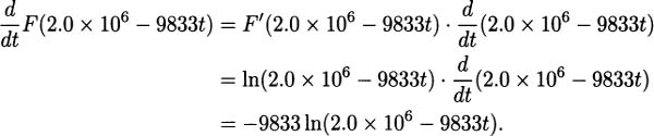
This would be exactly right, except for the extra constant factor of –9833 in front. Hopefully, you see that we can make one last adjustment, dividing by the constant –9833 to get an antiderivative that works perfectly. The antiderivative we need is

Wow, that was work! But it was work that brings us to our final goal. We can now integrate the velocity to find the position of the rocket at any time t.
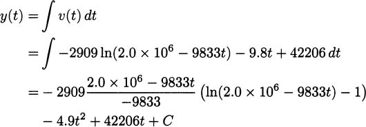
To discover the value of C, simply observe that the rocket begins on the ground. So when t = 0, the height of the rocket is y(0) = 0. It might be best to use a calculator for this part:
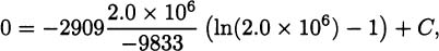
and, solving,
That makes the height function of the rocket

To calculate the height of the rocket after two minutes (which is 120 seconds), evaluate y(120) to get approximately 62,000 meters. Is this a reasonable answer?
Let’s convert it to miles:
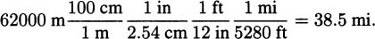
If we check our numbers against NASA results, NASA says that after about 2 minutes of flight, the space shuttle has finished its first stage. It is at a height of 28 miles, and it is traveling 3000 mph. We computed a height of 38.5 miles and (in the previous section) a velocity of 3172 mph. It’s not a perfect match, but we are pretty close.
If you feel bad that our conclusion was off by about 10 miles, it may console you to know that at 3000 mph, the space shuttle covers 10 miles in approximately 12 seconds. So don’t think of our calculation as being off by 10 miles. Think of it as being off by 12 seconds.
4.90 Assume that the space shuttle has a mass of m = 2.0 × 10⁶ kg, and the engines produce F = 2.86 × 10⁷ kg m/s2 of force. For this exercise, imagine that the shuttle stays the same mass, rather than getting lighter as it expends fuel.
 , what is the velocity of the shuttle when 2 = 120 s?
4.91 Compute the derivative of each function.
4.92 Compute the derivative of each function.


4.93 Consider the height function we derived for the rocket:

Here’s a mathematical riddle. “I am a real number. I am not negative, but I am less than any positive number. Who am I?”
The answer, of course, is zero. But if we change the setting slightly, it can feel less obvious. For example, perhaps you are acquainted with the infinite repeating decimal number 1.999999… = 1. . Do you know what number this is? As a riddle, we might have said, “I am a real number. I am not greater than 2, but I am greater than any number less than 2. Who am I?” Naturally, the answer is 2. Yet for many people, it feels strange to say “One point nine-repeating is another way of writing the number 2.”
What do we mean when we write a number like 1.999999…? Remember that in our decimal number system, each place in a number has a corresponding value. In this number, the 1 digit is in the ones place. Then a 9 follows in the tenths place, another 9 in the hundredths place and so on. Just as the number 9.81 means 9 +  , the expression 1.999999… means
If you think there might be something shifty about adding up infinitely many values, consider that in another context this probably doesn’t upset you at all. You are probably comfortable with the fact that 1/3 = 0.333333… = 0. , and 1/7 =
  . If you think about what those decimal expansions mean, each must refer to an infinite sum.
An infinite sum is called a series. Our goal is to find the sum of different kinds of series, including the series for 1. and 0.. As a step toward that goal, consider this version of Zeno’s famous dichotomy paradox: Imagine yourself standing on the number line. You are at the number 0 and facing towards the 1. Now step half the distance to 1. This puts you on 1/2. Step half the distance again, to 3/4. Step half the distance again, and again, and so on, forever. Where do you end up?
Hopefully, you see that, in the language of our riddle, you end up at a real number no larger than 1 but beyond any of the numbers less than 1. That is, you are at the number 1. As a series, this conclusion could be written as
To be very careful about this, however, consider where you are after each step. After your first step (of size 1/2), your distance from 1 was also 1/2. After your second step, (of size 1/4 = 1/22), you were at 3/4 and your distance from 1 was only 1/4 = 1/22. Each step is half as large as the previous, so the nth step is of size l/2n and it leaves you short of 1 by a distance of only l/2n. As n becomes larger and larger, you get closer and closer to 1 (though you never reach it in any finite number of steps). In the language of calculus, we solve the riddle by taking a limit, and here the limit is 1.
Mathematically, the sum of a series is always defined this way. We add up a finite (but ever growing) number of terms, then see if the finite sums approach some limit. If they do, the series is said to be convergent, and the limit is called the sum of the series.
The series  , and 1. are all members of an important family of (convergent) series, the geometric series. A geometric series is a series of the form

The Zeno series corresponds to a = 1/2 and r = 1/2. The value 0. corresponds to a = 3/10 and r = 1/10. The value 1. is not a geometric series, but the decimal part, 0., is a geometric series with a = 9/10 and r = 1/10.
Since the sum of a series comes from taking a limit of finite sums, it is important to be able to compute finite sums. For the geometric series, the finite sums are given by a well known formula.
There are two typical ways to derive this fact. If you are comfortable with polynomial long division, then computing  is a matter of dividing rn – 1 by r – 1. Otherwise, this formula can be checked by computing the product
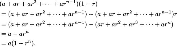
Since  , we can divide both sides by (1 – r) to get the finite sum formula.
Now that we know how to add finite geometric sums, we can ask what happens when n approaches infinity. The most interesting case is when |r| < 1, since in that case rn gets closer and closer to 0. To see this, consider any number of size (absolute value) less than 1. If you square your number and cube it, and so on, it becomes smaller and smaller.
Since rn → 0, we now know the limit of a geometric series.
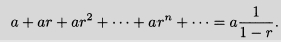
EXAMPLE 4.47The Zeno series is a geometric series with a = 1/2 and r = 1/2. The sum of the series, therefore, is
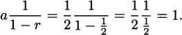
EXAMPLE 4.48The value 0. represents a geometric series with a = 3/10 and r = 1/10. The sum is therefore
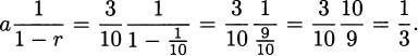
EXAMPLE 4.49The value 1. is not a geometric series, but 0. is. Here a = 9/10 and r = 1/10. The sum of the series part is
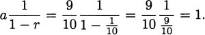
And finally, the value is 1. = 1 + 0. = 1 + 1 = 2.
EXAMPLE 4.50What value does x = 0. = 0.13131313… represent?
Solution: This question is slightly harder, but one way to write this as a series is
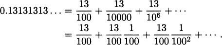
This is a geometric series with  and
and  . The sum is
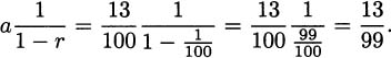
Here’s another approach, using algebra. Let x = 0.. Our job is to find x. Notice that lOOx = 13.131313… = 13.. Now compute:
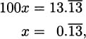
and subtracting.

Solving, we see again that x = 13/99.
Are there series that don’t converge? Of course. The simple series 1 + 1 + 1 + o o o fails to converge. Rather than getting close to any fixed number, it becomes larger and larger as you take more terms. Such a series is called divergent. In this example, we say that the series “diverges to infinity.”
It is fairly clear that if the terms of a series don’t get smaller and smaller, the series will be divergent. But what if the terms do get smaller? Is that enough to make the series converge? As it turns out, there are divergent series whose individual terms get smaller and smaller. The most famous is the harmonic series.
As always, the key to understanding the limit of any series is to look at n terms, and then see what happens as n gets larger and larger. If we take the first n terms of the harmonic series, we get  .
.
To see how big this sum is, we’ll use a geometric argument. Draw rectangles having area , and stack them next to each other on the number line, starting at the value x = 1, as indicated by the five rectangles in Figure 4.38. The jth rectangle should have width 1 and height  , so that each area is the jth term of the harmonic series.
Figure 4.38 The harmonic series as areas of rectangles.
Now that we are thinking of this sum as an area, our knowledge of calculus and integrals can be applied. Notice what happens if we insert the curve y = l/x into the picture, as in Figure 4.39.
Figure 4.39 Harmonic series compared with y = l/x.
Look first at what happens on the interval [1,2]. On this interval, we know that y = l/x will never be larger that 1. So, the area of the rectangle is larger than the area under the curve. In the language of integrals, we can write
The same thing happens in the next interval. In [2,3], we know that y = 1/x will never be larger than  , which is precisely the height of the second rectangle. So the area under the curve is smaller than the area of the rectangle. If we combine this with what we know about the first rectangle, we find that the sum of the first two rectangles is more than the area under the curve over the interval [1,3]:
We can continue in the same way. The area of five rectangles is greater than the area under the curve over the interval [1,6]. In general, the area of n rectangles will be greater than the area under y = 1/x over the interval [1, n + 1]. Written out,
Here’s the point. We know how to compute the area under the curve, because we know how to do integrals. All we need is an antiderivative for f(x) = 1/x, and F(x) = In x works fine. Applying the Fundamental Theorem of Calculus,

What does this tell us about the harmonic series? If we take n terms and add them together, it is true that we don’t know exactly what the result will be. But we do know that whatever that sum is, it will be more than ln(n + 1). Since ln(n + 1) goes to infinity as n gets larger, the harmonic series must also go to infinity as n grows.
4.94 Let x = 0.24 = 0.24999….
4.95 Write 2. = 2.222… as a fraction.
4.96 Write 0. = 0.123123123… as a fraction in lowest terms.
4.97 Interpret this math joke.
An infinite number of mathematicians walk into a bar. The first mathematician says to the bartender, “I’d like 1 glass of beer.” The second mathematician says, “I’d like 1/2 glass of beer.” The third mathematician says, “I’d like 1/4 glass of beer.” At that point, the bartender gets annoyed, slams a couple of mugs on the bar, and says, “Look. Here’s two glasses of beer. Now you all get out of here!”
If you’ve studied science, you may know that radioactive substances have a “half life,” a period during which half of the substance will decay into another element. For example, Polonium-210, which is used as a detonator for nuclear bombs, has a half-life of 138 days. After 138 days, a 1 gram sample of Polonium-210 decays until half of it is lead. After another 138 days, half of the remaining Polonium-210 will have decayed into lead (meaning that there is only 1/4 gram of Polonium-210 left in the sample). An expensive aspect of maintaining a large nuclear arsenal is continuously replacing decayed detonators.
If you’ve studied finance (or worked Exercise 4.64), you may know that compound interest endows investments with a doubling time. You might have learned the “rule of 72,” which estimates how long it takes for your money to double. According to the rule, if you divide 72 by your compound interest rate, the result is approximately the doubling time. For example, if you earn 6% on your money, it should double in 72/6 = 12 years.
Although the rule of 72 is often a good estimate, as math students, we can compute doubling times precisely. Let P be the amount of principal invested, and assume it grows at 6%, compounded annually. Then the amount of money after t years, A(t), is given by the formula
If we want to know when the investment will double, we simply set A(t) = 2P and find t. Calculating,
and to solve this, we take a logarithm of both sides,
Finally, we divide by In 1.06 to get t:
A similar calculation works with any investment that pays compound interest. That’s because compound interest is an example of exponential growth, and anything that grows exponentially has a doubling time. To see this, let A(t) = Pat be a generic exponential function with base a > 1 (it doesn’t grow if a < 1). Then we can compute the time it takes for doubling:

and, using logarithms, as before,

You can verify that the time required to go from 2P to 4P is of the same duration, as is the time to go from 3P to 6P, etc.
Other than compound interest, can you think of anything else that grows exponentially? Anything that “grows by a percentage” is exponential growth. For example, over the long term inflation is expected to grow around 3% per year. That means if an item costs $10 this year, it costs 3% more money a year from now, or $10 + $10(0.03) = $10(1.03) = $10.30. In two years, the cost is $10(1.03)2, and after t years the cost is $10(1.03)t.
Population is another quantity that often grows exponentially. Some percentage of the population tends to be older (or die randomly from accidents). Another percentage is of childbearing age and temperament to have offspring. The difference is the growth rate of the population. It fluctuates, but over the long term it has tended to have an exponential shape.
Figure 4.40 shows government estimates for the amount of fossil fuel used in the United States since 1900. The curve through the data points has the formula f(t) = e2.48+0.0221t = 11.9e0.0221t, which we recognize as an exponential curve.
If fossil fuel use has grown (approximately) exponentially, it should have a doubling time, and we can calculate it. First, f(0) = 11.9, since fossil fuel use in 1900 was approximately 11.9 quadrillion British thermal units. To find the doubling period, we solve to find the t for which fuel use had doubled to 23.8 quadrillion BTUs:
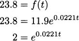
and taking logs of both sides,
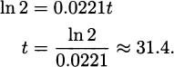
In the United States over the last century, fossil fuel use doubled approximately every 31.4 years. Is that an alarming rate? Perhaps not: the growth rate might be thought leisurely at only a bit over 2% per year. Yet there are some reasons to think it is alarming, and our knowledge of series can give us some perspective on the question.
Figure 4.40 US fossil fuel use since 1900.
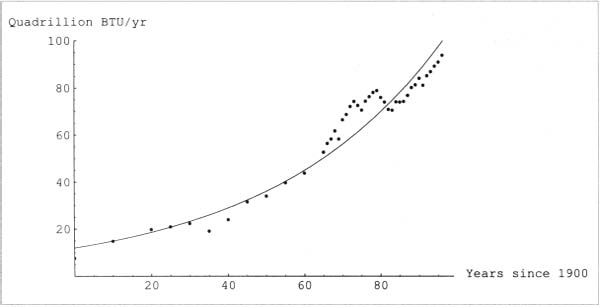
Let x be the total amount of fossil fuel used in one doubling period (in this case 31.4 years). How much was used during the period before? If you answered  , you are correct. How much was used during the period before that? Yes,
  . Looking backward, counting by doubling times, we get a progression that looks like a geometric series, as in Figure 4.41.
Figure 4.41 Fossil fuel use divided into doubling periods.
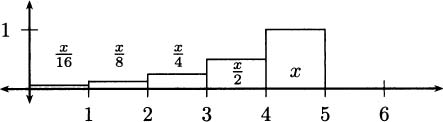
Compare the amount of fuel used in the final doubling period to the periods that came before. What happens if we start adding the previous amounts? We get
This is a finite part of a geometric series, with a = and r = . four terms is less than the sum of the entire series, which we can calculate:
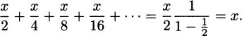
What did we learn? Not only is the amount of fossil fuel used in the final doubling period equal to twice as much as the preceding period, it is more than all of previous history added together. If this kind of growth continues, what will happen during the next doubling period? In Figure 4.42 the final doubling period again exceeds all of previous history, and that includes the period we just finished!
Figure 4.42 Fossil fuel use after one more doubling period.
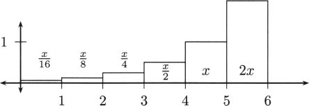
Exponential growth negates many arguments for complacency about energy policy. For example, what if there are twice as many resources as we estimate still in the ground, coal and oil and gas still undiscovered and untapped? That buys us more time, but not hundreds of years, merely one more 31.4 year doubling period. It is clear that repeatedly doubling consumption is not a pattern that can continue indefinitely.
EXAMPLE 4.51The United Nations has estimated that the world human population was approximately 6 billion in the year 2000 and was increasing at the rate of approximately 1 percent per year at that time. Based on this information, find the function representing world human population as a function of the number of years past 2000. When will population reach 10 billion, according to this model?
Solution: Let A(t) be the world human population at time t, where t is number of years after 2000. Since population grows by a percentage, we recognize it as exponential growth, and we can write A(t) = Pert for some value of P and some value of r. We are told that the population in 2000 is 6 billion, thus 6 × 109 = A(0) = Per·0 = P, and it follows that A(t) = 6 × 10⁹ ert.
We are also told that the rate of change of population is 1 percent per year. Since derivatives tell us rates of change, this means that
and substituting for A(t), we have
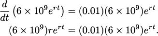
Divide both sides by 6 × 10⁹ ert to get

Therefore, the model for global population growth is
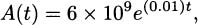
and to find the time when A(t) = 1010 we solve the equation
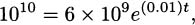
obtaining t ≈ 51. The world’s human population will reach 10 billion in the year 2051, according to this model.
4.98 Suppose that you have a bank account earning 5 percent interest per year, compounded annually. If you have $2000 today, when will you have $4000?
4.99 Assume the inflation rate remains 3.4% per year.
In this chapter we have seen that calculus is the mathematics we use to understand change. When quantities change, derivatives tell us the rate. If we know a rate, integrals allow us to transform that knowledge into a total change. Our study has allowed us to maximize and minimize functions, to analyze the history of fossil fuel use, and even to compute (roughly) the height of a rocket.
Yet as much as we have learned, our view of calculus has been very one-dimensional, literally. We worked solely with functions of a single variable. The world is filled with beautiful complicated things that can’t be expressed as functions of one variable. For example, when a rocket launches into orbit, it doesn’t fly straight up as we assumed in Section 4.17. It follows some arc into space that results in an elliptical shaped orbit. Truly modeling the height of a rocket requires a three-dimensional view and functions with variables x, y, z, and t, along with corresponding multidimensional calculus principles. There are whole courses of study that take the ideas of calculus and put them in a multi-variable context.
Many of the physical models we use for the universe around us are based on relationships defined in terms of derivatives. For example, Newton’s Law of Cooling says that the rate of change in the temperature of an object is proportional to the difference in temperature between the object and its surroundings. Informally, it says that very hot objects cool at a faster rate than slightly hot objects (but it still takes hot objects longer to completely cool since they have further to go). Formally, Newton’s Law of Cooling is a differential equation, an equation containing derivatives of a function,
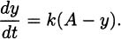
To solve a differential equation is to find a function y that makes the equation true. For example, in the equation above, y = y(t) = A + Be–kt works. Take a derivative for yourself and check. After a first course in calculus, many people go on to one or more courses in differential equations.
One can also study calculus where the functions are defined on the complex numbers (i.e., numbers that have both real and imaginary parts). The complex numbers are an especially beautiful domain in which to do calculus, and many elegant results exist in this context. One elegant fact is that any function that has a (single) derivative defined at every complex number is guaranteed to have a power series, which is a way of saying that it can be written as an infinite polynomial. For example, the exponential function has a power series,
Calculus has helped us gain understanding in nearly every domain of mathematics, including number theory, geometry, game theory, topology, numerical analysis, and probability. It is an essential tool for physics, chemistry, biology, engineering, economics, and statistics. It is one of humankind’s most powerful and awe-inspiring creations.
4.100 Let y(t) = 70 + 20e–2t, which might describe the temperature of an object that cools from 90°F to room temperature at 70°F.
 and verify that you get the same answer as in part (a).
4.101 Let y(t) = A + Be–kt, where A, B, and k are constants.
and verify that you get the same answer as in part (a).4.102 Let  terms in the power series for ex.
1W. M. Priestley, “Sherlock Holmes Meets Pierre de Fermat,” Calculus: A Liberal Art, second edition, Springer-Verlag, New York, 1998.