CHAPTER 8

Optical Spectra

8.1 General Remarks

A spectrum may be defined as an ordering of electromagnetic radiation according to frequency, or what amounts to the same thing, an ordering by wavelength. The complete spectrum of a given source comprises all the frequencies that the source emits. Since no single universal frequency-resolving instrument exists, the various regions of the electromagnetic spectrum must be investigated by different methods. The main regions have already been mentioned in Section 1.4.

The so-called “optical” region extends over a wide range from the far infrared on the one end to the far ultraviolet on the other. It includes the visible region as a relatively small portion (Figure 8.1).

Figure 8.1. The optical region of the electromagnetic spectrum.

In practice the optical region is characterized by (1) the fact that the radiation is focused, directed, and controlled by mirrors and lenses, and (2) the use of prisms and gratings for dispersing the radiation into a spectrum.

Unlike the continuous spectrum of thermal radiation given off by solid bodies, the radiation emitted by excited atoms or molecules is found to consist of various discrete frequencies. These frequencies are characteristic of the particular kinds of atoms or molecules involved. The term “line” spectrum is commonly used when referring to such radiation. This terminology originates from the fact that a slit is generally the type of entrance aperture for spectroscopic instruments used in the optical region, so a separate line image of the slit is formed at the focal plane for each different wavelength comprising the radiation. Sources of line spectra include such things as arcs, sparks, and electric discharges through gases.

The optical spectra of most atoms are quite complex and the line patterns are seemingly random in appearance. A few elements, notably hydrogen and the alkali metals, exhibit relatively simple spectra that are characterized by easily recognized series of lines converging toward a limit.

The optical spectra of many molecules, particularly diatomic molecules, appear as more or less regularly spaced “bands” when examined with a spectroscopic instrument of low resolving power. However, under high resolution, these bands are found to be sequences of closely spaced lines.

When white light is sent through an unexcited gas or vapor, it is generally found that the atoms or molecules comprising the vapor absorb just those same frequencies that they would emit if excited. The result is that those particular frequencies are either weakened or are entirely missing from the light that is transmitted through the vapor. This effect is present in ordinary sunlight, the spectrum of which appears as numerous dark lines on a bright continuous background.

The dark lines are called Fraunhofer lines after J. Fraunhofer who made early quantitative measurements. These lines reveal the presence of a relatively cool layer of gas in the sun’s upper atmosphere. The atoms in this layer absorb their own characteristic wavelengths from the light coming from the hot, dense surface of the sun below, which emits thermal radiation corresponding to a temperature of about 5500°K.

Selective absorption is also exhibited by solids. Virtually all transparent solids show broad absorption bands in the infrared and ultraviolet. ln most colored substances these absorption bands extend into the visible region. However, relatively sharp absorption bands may occur in certain cases such as crystals and glasses that contain rare earth atoms as impurities.

8.2 Elementary Theory of Atomic Spectra

The mathematical theory of atomic spectra had its beginning in 1913 when Niels Bohr, a Danish physicist, announced his now famous work. He was concerned mainly with a theoretical explanation of the spectrum of hydrogen, although his basic ideas are applicable to other systems as well.

In order to explain the fact that atoms emit only certain characteristic frequencies, Bohr introduced two fundamental assumptions. These are

1. The electrons of an atom can occupy only certain discrete quantized states or orbits. These states have different energies, and the one of lowest energy is the normal state of the atom, also known as the ground state.
2. When an electron undergoes a transition from one state to another, it can do so by emitting or absorbing radiation. The frequency v of this radiation is given by
   

   (8.1)

   where ΔE is the energy difference between the two states involved, and h is Planck’s constants.

These assumptions represent a radical departure from the classical or Newtonian concept of the atom. The first is suggestive of the quantization of cavity radiation introduced earlier by Planck. The second idea amounts to saying that an atom emits, or absorbs, a single photon upon changing from one quantized state to another, the energy of the photon being equal to the energy difference between the two states (Figure 8.2).

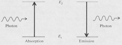
Figure 8.2. Diagram showing the processes of absorption and emission.

The frequency spectrum of an atom or molecule is given by taking the various possible energy differences ∣E₁ — E₂∣ and dividing by h. In order to calculate the actual spectrum of a given atom, one must first know the energies of the various quantum states of the atom in question. Conversely, the energies of the quantum states can be inferred from the measured frequencies of the various spectrum lines.

The Bohr Atom and the Hydrogen Spectrum In his study of the hydrogen atom, Bohr was able to obtain the correct formula for the energy levels by introducing a fundamental postulate concerning angular momentum. According to this postulate, the angular momentum of an electron is always an integral multiple of the quantity h/2π, where h is Planck’s constant.

An electron of mass m traveling with speed u in a circular orbit of radius r has angular momentum mur. Hence the relation

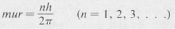
(8.2)

expresses the quantization of the orbital angular momentum of the electron. The integer n is known as the principal quantum number.

The classical force equation for an electron of charge —e revolving in a circular orbit of radius r, centered on a proton of charge +e, is

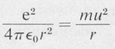
(8.3)

By elimination of u between the two equations, one obtains the following formula for the radii of the quantized orbits:

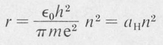
(8.4)

The radius of the smallest orbit (n = 1 ) is called the first Bohr radius and is denoted by a_H. Its numerical value is

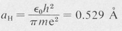
(8.5)

The various orbits are then given by the sequence a_H, 4a_H, 9a_H, ... , and so forth.

The total energy of a given orbit is given by the sum of the kinetic and the potential energies, namely,

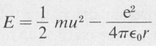
(8.6)

Eliminating u by means of Equation (8.3) one finds

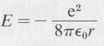
(8.7)

This is the classical value for the energy of a bound electron. If all values of r were allowed, then any (negative) value of energy would be possible. But the orbits are quantized according to Equation (8.4). The resultant quantized energies are given by

(8.8)

in which the constant R, known as the Rydberg constant, is

(8.9)

This is also the binding energy of the electron in the ground state, n = 1. Its value in electron volts is approximately 13.5 eV.

The formula for the hydrogen spectrum is obtained by combining the energy equation with the Bohr frequency condition. Calling E₁ and E₂ the energies of the orbits n₁ and n₂, respectively, we find

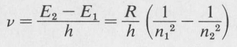
(8.10)

The numerical value of R/h is 3.29 x 10¹⁵ Hz.¹

A transition diagram of the hydrogen atom is shown in Figure 8.3. The energies of the various allowed orbits are plotted as horizontal lines, and the transitions, corresponding to the various spectral lines, are shown as vertical arrows. Various combinations of the integers n₁ and n₂ give the observed spectral series. These are as follows:

n1=1	n2=2, 3, 4, . . .	Lyman series (far ultraviolet)
n1=2	n2=3, 4, 5, . . .	Balmer series (visible and near ultraviolet)
n1=3	n2=4, 5, 6, . . .	paschen series (infrared)
n1=4	n2=5, 6, 7, . . .	Brackett series (infrared)
n1=5	n2=6, 7, 8, . . .	pfund series (infrared)
.

Some of the series are shown in Figure 8.4 on a logarithmic wavelength scale.

The first three lines of the Balmer series, namely, H_α at a wavelength of 6563 Å, H_β at 4861 Å, and H_γ at 4340 A, are easily seen by viewing a simple hydrogen discharge tube through a small spectroscope. The members of the series up to n₂ = 22 have been recorded by photography. The intensities of the lines of a given series diminish with increasing values of n₂. Furthermore, the intensities of the various series decrease markedly as n₁ increases. Observations using ordinary laboratory sources have extended as far as the line at 12.3 μ in the infrared, corresponding to n₁ = 6, n₂ = 7.

¹ Spectroscopists usually write Equation (8.10) in terms of spectroscopic wavenumber

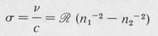
where ℛ is the Rydberg constant in wavenumber units, namely,

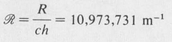
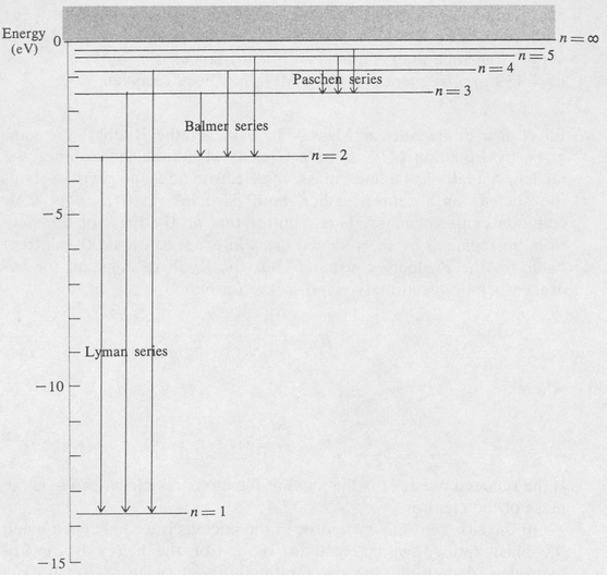
Figure 8.3. Energy levels of atomic hydrogen. Transitions for the first three series are indicated.

The hydrogen spectrum is of particular astronomical importance. Since hydrogen is the most abundant element in the universe, the spectra of most stars show the Balmer series as prominent absorption lines. The series also appears as bright emission lines in the spectra of many luminous nebulas. Recent radiotelescope observations [26] have revealed interstellar hydrogen emission lines corresponding to very large quantum numbers. For instance, the line n₁ = 158, n₂ = 159 at a frequency of 1651 MHz has been received.

Figure 8.4. The first three series of atomic hydrogen on a logarithmic wavelength scale.

Effect of a Finite Nuclear Mass The value of the Rydberg constant given by Equation (8.9) is for a nucleus of infinite mass. Since the nucleus actually has a finite mass, the electron does not revolve about the nucleus as a center, rather, both particles revolve about their common center of mass. This requires that m, the mass of the electron, be replaced by the reduced mass in order to obtain the correct value for the Rydberg constant. Thus the Rydberg constant for hydrogen is more accurately given by the formula

(8.11)

where

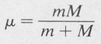
(8.12)

is the reduced mass, M is the mass of the atomic nucleus, and m is the mass of the electron.

In the case of ordinary hydrogen the nucleus is a single proton and the mass ratio M/m is equal to 1836. For the heavy isotope of hydrogen, deuterium, the mass ratio is about twice as much. The Rydberg constant for deuterium is therefore slightly different from that for hydrogen. The result is that a small difference exists between the frequencies of corresponding spectrum lines of the two isotopes. This effect, called isotope shift, can be seen as a “doubling” of the lines from a discharge tube containing a mixture of hydrogen and deuterium.

The Bohr model of the hydrogen atom, although giving essentially correct numerical results, is unable to account for the fact that the electron does not radiate while traveling in its circular orbit in the ground state, as required by classical electromagnetic theory. Further, the theory is difficult to apply to more complicated atoms and is completely inapplicable to molecules. Early attempts were made by various theorists to modify Bohr’s theory in order to account for such things as the fine structure of spectrum lines, and so forth (Section 8.7, below). These attempts met with varying degrees of success. However, the Bohr theory has now been superseded by the modern quantum theory of the atom, which will be discussed in the following sections.

Spectra of the Alkali Metals An empirical formula similar to that for hydrogen gives fairly accurate results for the spectra of the alkali metals lithium, sodium, and so forth. This formula is

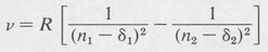
(8.13)

The Rydberg constant R is approximately the same as R _H. It has a slightly different value for each element. The quantum numbers n₁ and n₂ are integers, and the associated quantities δ₁ and δ₂ are known as quantum defects.

In a given spectral series, specified by a fixed value of n₁ and a sequence of increasing values of n₂, the quantum defects are very nearly constant. The most prominent series for the alkalis are designated as sharp, principal, diffuse, and fundamental, respectively. As a typical example, the quantum numbers and quantum defects for the series in sodium are listed in Table 8.1.

Table 8.1. SERIES IN SODIUM

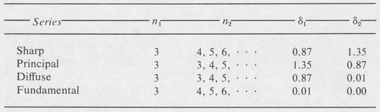
The sharp and the diffuse series are so named because of the appearance of the spectral lines.

The principal series is the most intense in emission and is also the one giving the strongest absorption lines when white light is passed through the vapor of the metal.

In the case of the fundamental series, the quantum defects are very small. As a consequence the frequencies of the lines of this series are very nearly the same as those of the corresponding series in hydrogen. This is the reason for the name “fundamental.”

8.3 Quantum Mechanics

Modern quantum theory was pioneered by Schrödinger, Heisenberg, and others in the 1920s. Originally there were two apparently different quantum theories called wave mechanics and matrix mechanics. These two formulations of quantum theory were later shown to be completely equivalent. Quantum mechanics, as it is known today, includes both. We shall not attempt a rigorous development of quantum mechanics here, but shall merely state some of the essential results that apply to atomic theory.

The quantum mechanical description of an atom or atomic system is made in terms of a wave function or state function. The commonly used symbol for this function is Ψ. Ordinarily Ψ is a complex number and is considered to be a function of all of the configurational coordinates of the system in question including the time.

According to the basic postulates of quantum mechanics, the state function Ψ has the property that the square of its absolute value, |Ψ|² or Ψ * Ψ, is a measure of the probability that the system in question is located at the configuration corresponding to particular values of the coordinates. Ψ * Ψ is sometimes referred to as the probability distribution function or the probability density.

If the system is a single electron, for example, with coordinates x, y, and z, then the probability that the electron is located between x and x + Δx, y and y + Δy, z and z + Δz is given by the expression

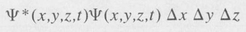
(8.14)

It is evident from the above interpretation of the state function that one can never be certain that the electron is located at any given place. Only the chance of its being there within certain limits can be known. This is entirely consistent with the Heisenberg uncertainty principle discussed earlier in Section 7.11.

Now the total probability that the electron is located somewhere in space is necessarily unity. It follows that the integral, over all space, of the probability density is finite and has, in fact, the value 1, namely,

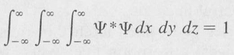
(8.15)

Functions satisfying the above equation are said to be quadratically integrable, normalized functions.

Stationary States A characteristic state or eigenstate is one that corresponds to a perfectly defined energy. A given system may have many eigenstates, each possessing, in general, a different energy. If E_n denotes the particular energy of a system when it is in one of its characteristic states, then the time dependence of the state function is given by the complex exponential factor exp (–iE_n t/ħ), where

Consequently the complete state function is expressible as

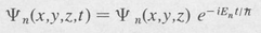
(8.16)

Here ψ_n is a function of the configurational coordinates only. It does not involve the time.

Consider the probability density of a system in one of its characteristic states. We have

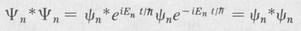
(8.17)

We see that the exponential factors cancel out. This means that the probability distribution is constant in time, or stationary. Thus characteristic states are also called stationary states. A system that is in a stationary state is a static system in the sense that no changes at all are taking place with respect to the external surroundings.

In the particular case in which the quantum-mechanical system is an atom, consisting of a nucleus with surrounding electrons, the probability distribution function is actually a measure of the mean electron density at a given point in space. One sometimes refers to this as a charge cloud. When an atom is in a stationary state, the electron density is constant in time. The surrounding electromagnetic field is static and the atom does not radiate.

Coherent States Consider a system that is in the process of changing from one eigenstate ψ₁ to another ψ₂. During the transition the state function is given by a linear combination of the two state functions involved, namely,

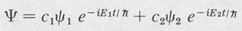
(8.18)

Here c₁ and c₂ are parameters whose variation with time is slow in comparison with that of the exponential factors. A state of the above type is known as a coherent state. One essential difference between a coherent state and a stationary state is that the energy of a coherent state is not well defined, whereas that of a stationary state is.

The probability distribution of the coherent state represented by Equation (8.18) is given by the following expression:

(8.19)

where

(8.20)

or, equivalently,

The above result shows that the probability density of a coherent state undergoes a sinusoidal oscillation with time. The frequency of this oscillation is precisely that given by the Bohr frequency condition.

The quantum-mechanical description of a radiating atom may be stated as follows: During the change from one quantum state to another, the probability distribution of the electron becomes coherent and oscillates sinusoidally; this sinusoidal oscillation is accompanied by an oscillating electromagnetic field that constitutes the radiation.

8.4 The Schrödinger Equation

Thus far we have not discussed the question of just how one goes about finding the state functions of a particular physical system. This is one of the basic tasks of quantum theory, and the performance of this task involves the solution of a differential equation known as the Schrödinger equation. A simple derivation of this important equation for the case of a single particle proceeds as follows.

Consider any wave function Ψ whose time dependence has the usual sinusoidal variation. Let λ be the wavelength. Then we know that the spatial part ψ of the wave function must obey the standard time-independent wave equation

Now according to de Broglie’s hypothesis (Section 7.10), a particle having momentum p has an associated wavelength h/p. Thus a particle would be expected to obey a wave equation of the form

But a particle of mass m has energy E given by E = mu² + V, in which V is the potential energy and u is the speed. Since the linear momentum p = mu, then

p²= 2m(E–V)

The wave equation of the particle can therefore be written as

(8.21)

This is the famous equation first announced by Erwin Schrödinger in 1926. It is a linear, partial differential equation of the second order. The physics involved in the application of the equation essentially amounts to the selection of a potential function V(x,y,z) appropriate to the particular physical system in question. Given the potential function V(x,y,z), the mathematical problem is that of finding the function (or functions) ψ which satisfy the equation.

Not all mathematical solutions of the Schrödinger equation are physically meaningful. In order to represent a real system the function ψ must tend to zero for infinite values of the coordinates in such a way as to be quadratically integrable. This has already been implied by Equation (8.15).

The details of solving partial differential equations of the Schrödinger type are often very involved and complicated, but the results are easily understood. It turns out that the requirement that the solutions be quadratically integrable leads to the result that acceptable solutions can exist only if the energy E has certain definite values. These allowed values of E, called eigenvalues, are, in fact, just the characteristic energy levels of the system. The corresponding solutions are called eigenfunctions. They are the state functions of the system.

The Schrödinger equation thus leads to the determination of the energy states of the system as well as the associated state functions. In the next section it is shown how the Schrödinger equation is applied to the problem of calculating the energy levels and state functions of the hydrogen atom.

8.5 Quantum Mechanics of the Hydrogen Atom

The quantum theory of a single electron moving in a central field, briefly outlined here, forms the basis of modern atomic theory. In the mathematical treatment of the one-electron atom it is convenient to employ polar coordinates r, θ, and φ, owing to spherical symmetry of the field in which the electron moves. The Laplace operator in these coordinates is

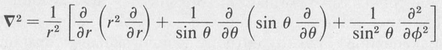
(8.22)

The corresponding Schrödinger equation is

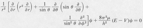
(8.23)

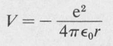
Here μ is the reduced mass of the electron. In the case of the hydrogen atom, the potential V is given by

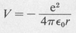
(8.24)

Ground State of the Hydrogen Atom We shall first obtain a simple solution of the Schrödinger equation by the trial method. Substituting a simple exponential trial solution of the form

(8.25 )

where α is an undetermined constant, we find that the Schrödinger equation reduces to

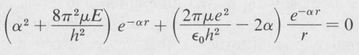
(8.26)

This equation can hold for all values of r only if each expression enclosed by parentheses vanishes, namely,

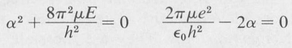
(8.27)

The second equation gives the value of α. We find that it turns out to be just the reciprocal of the first Bohr radius:

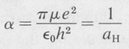
(8.28)

Substituting this value of α into the first equation and solving for E, we obtain

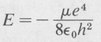
(8.29)

This is identical with the value of the energy of the first Bohr orbit, obtained in Section 8.3. It is the energy of the ground state of the hydrogen atom.

Now the solution given by Equation (8.25), in which α is given by Equation (8.28), does not yet represent a completely acceptable state function, for it is not normalized. But one can always multiply any solution by an arbitrary constant and still have a solution of the differential equation. Thus, by introducing a normalizing constant C, we can write

(8.30)

This does not affect the value of the energy E. The normalizing condition equation (8.23) reduces to

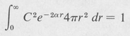
(8.31)

from which C may be found. If one is interested only in the spatial variation of the state function, it is not necessary to include the normalizing constant.

According to the above results the ground state of the hydrogen atom is such that the probability density of the electron is spherically symmetric and decreases exponentially with the radial distance r. The density is greatest at the center and diminishes by the factor e^–2 in a distance of one Bohr radius. A plot of the density function is shown in Figure 8.5.

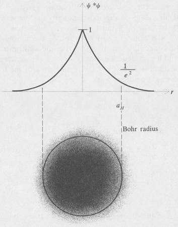
Figure 8.5. Probability density of the ground state (1s) of the hydrogen atom.

Excited States In order to find the state functions and the energies of the excited states of the hydrogen atom, it is necessary to solve the Schrödinger equation completely. To do this, the method of separation of variables is used.

The state function ψ is expressed as a product of three functions, a radial function and two angular functions, namely,

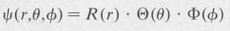
(8.32)

The Schrödinger equation (8.23) can then be written as

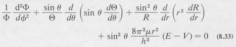
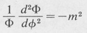
Now in order that our assumed solution satisfy the differential equation for all values of the independent variables r, θ, and φ, the first term (1/Φ) (d²Φ/dφ²) must necessarily be equal to a constant. Otherwise r and θ would be dependent on φ. We denote this constant by –m². The remaining equation can then be split into two parts, a radial part and a part dependent only on θ. Setting each part equal to a second constant, denoted by /(/ + I), one obtains the following separated differential equations:

(8.34)

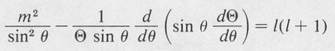
(8.35)

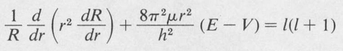
(8.36)

where, in the case of the hydrogen atom,

A solution of the differential equation (8.34) involving φ is clearly

(8.37)

In order for this to be a physically acceptable solution, it is necessary that Φ assumes the same value for φ, φ + 2π, φ + 4π, and so forth; otherwise, the state function would not be uniquely defined at a given point in space. This requirement restricts the allowed values of m to integers, namely,

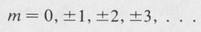
(8.38)

The number m is called the magnetic quantum number.

The θ-dependent equation (8.35) and the radial equation (8.36) are more difficult to solve. We shall not go into the details of their solution here, but shall merely give the results as given in any standard text on quantum mechanics. It happens that both differential equations were well known long before the time of Schrodinger. Their solutions had been worked out in connection with other problems in mathematical physics.

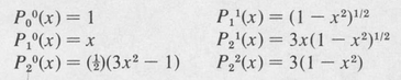
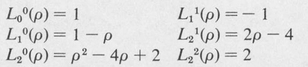
The equation in θ, Equation (8.35), is one form of an equation known as “Legendre’s differential equation.” This equation yields acceptable (single-valued) solutions only if l is a positive integer whose value is equal to or greater than ∣m∣. The integer / is called the azimuthal quantum number. The resulting solutions are known as associated Legendre polynomials, denoted byP_l^∣m∣ (cos θ). They may be found by means of a generating formula

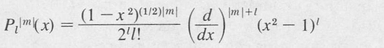
(8.39)

A few of these are:

The radial equation (8.36) is called “Laguerre’s differential equation.” Acceptable solutions (ones leading to quadratically integrable functions) are given by the formula

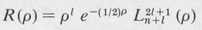
The variable ρ is defined as a certain constant times r, namely,

(8.40)

The quantity n is the principal quantum number. It is an integer whose value is equal to or greater than / + 1. The functions (ρ) are called associated Laguerre polynomials. A formula for generating them is

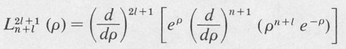
(8.41)

Some of these are as follows:

In the process of solving the radial differential equation, it is found that the eigenvalues of the energy E are determined solely by the principal quantum number n. The eigenvalues are given by the formula

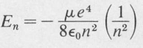
(8.42)

This is exactly the same formula as that given by the simple Bohr theory.

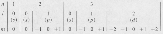
For each value of the principal quantum number n, with energy E_n given by the above equation, there are n different possible values of the azimuthal quantum number /, namely, 0, 1, 2, . . . , n–2, n — 1. Each value of / represents a different kind of eigenstate. States in which / = 0, 1, 2, 3 are traditionally called s, p, d, and ƒ states, respectively.

For each value of /, there are 2l + 1 possible values of the magnetic quantum number m. These are–l,–(l– 1), . . . ,–1, 0, + 1, . . . , +(/–1), +l. As a result, there are n² different eigenfunctions or states for each value of n. The following diagram summarizes the situation:

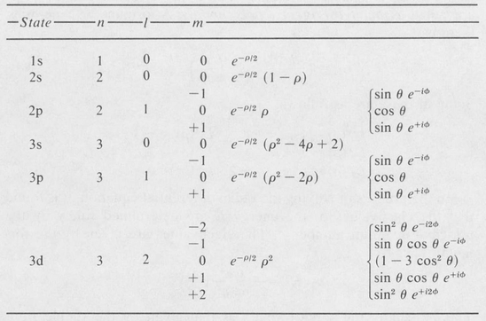
The complete state function, corresponding to prescribed values of n, /, and m, is given by the formula

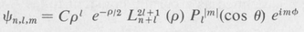
(8.43)

where ρ = 2r/na_H, and C is a normalizing constant. Table 8.2 shows a few of the simpler state functions of the hydrogen atom. Some of these are illustrated in Figure 8.6.

Table 8.2. EIGENFUNCTIONS OF THE HYDROGEN ATOM (NORMALIZING CONSTANTS OMITTED)

Angular Momentum The angular momentum of an electron moving in a central force field can be obtained by standard quantum-mechanical methods. It develops that the angular momentum is quantized, as in the Bohr theory, and that the magnitude is determined by the quantum numbers designating the various quantum states.

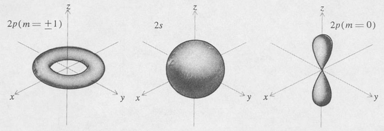
Figure 8.6. Probability density for the first excited state (n = 2) of the hydrogen atom.

The total orbital angular momentum is given by an expression involving only the azimuthal quantum number /, namely,

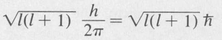
This is different from the value nh/2π of the Bohr theory. In particular, for s states (/ = 0), the angular momentum is zero. Physically this means that the electron cloud for s states does not possess a net rotation. It does not preclude any motion of the electron.

Theory also shows that the z component of the angular momentum is quantized. This component has the value

where m is the magnetic quantum number. As we have seen, m is the quantum number associated with the angle of rotation φ about the z axis. Since m can assume any of the values 0, ± 1, ±2, . . . , ±l, it follows that there are 2l + 1 different possible values of the z component of the angular momentum for a given value of l. This is illustrated in Figure 8.7.

8.6 Radiative Transitions and Selection Rules

As already mentioned, when an atom is in the process of changing from one eigenstate to another, the probability density of the electronic charge becomes coherent and oscillates sinusoidally with a frequency given by the Bohr frequency condition. The way in which the charge cloud oscillates depends on the particular eigenstates involved. In the case of a so-called dipole transition, the centroid of the negative charge of the electron cloud oscillates about the pos-itively charged nucleus. The atom thereby becomes an oscillating electric dipole.

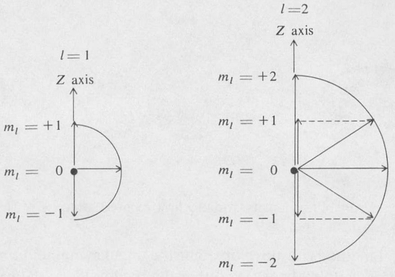
Figure 8.7. Space quantization of angular momentum for the cases l = 1 and L = 2.

Figure 8.8 is a diagram showing the time variation of the charge distribution for the hydrogen atom when it is in the coherent state represented by the combination 1s + 2p(m = 0). It is seen that the centroid of the charge moves back and forth along the z axis. The associated electromagnetic field has a directional distribution that is the same as that of a simple dipole antenna lying along the z axis. Thus the radiation is maximum in the xy plane and zero along the z axis. The radiation field in this case is linearly polarized with its plane of polarization parallel to the dipole axis.

A different case is shown in Figure 8.9. Here the coherent state is the combination 1s + 2p(m = + 1). The centroid of the electronic charge now moves in a circular path around the z axis. The angular frequency of the motion is also that given by the Bohr frequency formula ω = ΔE/π.

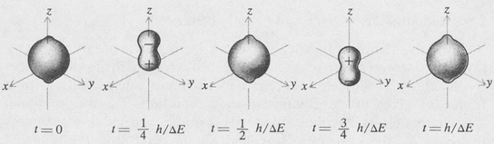
Figure 8.8. Charge distribution in the coherent state 1s + 2p₀ as a function of time. The atom is an oscillating dipole.

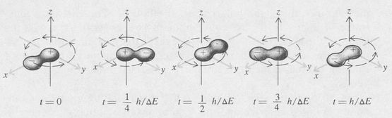
Figure 8.9. Charge distribution in the coherent state 1s + 2p₁ as a function of time. The atom is a rotating dipole.

Instead of an oscillating dipole, the atom is now a rotating dipole. The associated radiation field is such that the polarization is circular for radiation traveling in the direction of the z axis and linear for radiation traveling in a direction perpendicular to the z axis. For inter-mediate directions, the polarization is elliptical. The cases are illustrated in Figure 8.10. The coherent state 1s + 2p(m =–1) is just the same as the state 1s + 2p(m = + 1) except that the direction of rotation of the electronic charge is reversed. Consequently, the sense of rotation of the associated circularly polarized radiation is also reversed.

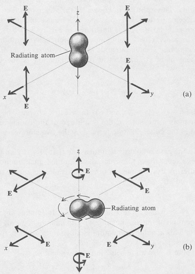
Figure 8.10. Polarization of the associated electromagnetic radiation (E vector) for (a) an oscillating dipole and (b) a rotating dipole.

In an ordinary spectral-light source the radiating atoms are randomly oriented in space and their vibrations are mutually incoherent. The total radiation is thus an incoherent mixture of all types of polarization. In other words the radiation is unpolarized. However, if the source is placed in a magnetic field, the field provides a preferred direction in space–the z axis in the above discussions [Figure 8.11(a)]. In addition the interaction between the radiating electron and the magnetic field causes each energy level to become split into several sublevels–one for each value of the magnetic quantum number m. As a result each spectrum line is split into several components. This splitting is known as the Zeeman effect. By means of the Zeeman effect, it is possible to observe the polarization effects mentioned above. This is illustrated in Figure 8.11(b).

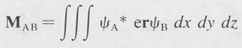
The general theory of atomic emission and absorption involves the calculation of certain integrals known as matrix elements. The matrix element involved in electric dipole radiation is the quantity M_AB defined as

(8.44)

where , and e is the electric charge. The dipole matrix element is a measure of the amplitude of the oscillating dipole moment of the coherent state formed by the two stationary states ψ_A and ψ_B.

In the case of hydrogen it turns out that M_AB is zero for all pairs of states except those for which the azimuthal quantum numbers l_A and /_B differ by exactly one. In other words electric dipole transitions are “allowed” if

(8.45)

This is known as the l-selection rule . It implies that the angular momentum of the atom changes by an amount ħ during a dipole transition. This angular momentum is taken up by the photon involved in the transition.

There is also an m-selection rule, which is

(8.46)

Transitions for which Δm = 0 are of the simple linear-dipole type, whereas those for which Δm = ± 1 are associated with a rotating dipole. The two types of transition are, in fact, those just discussed for hydrogen and illustrated in Figure 8.11.

Figure 8.11. The Zeeman effect. Simplified diagram which neglects electron spin. (a) Direction of the external magnetic field; (b) transition diagram. For light that is emitted in a direction perpendicular to the magnetic field, there are three components that are linearly polarized as shown. There are only two components for the light emitted to the field, and these are circularly polarized as indicated. The fundamental Zeeman splitting is Δν = eH/4πμ₀m, where H is the magnetic field, e is the electronic charge, and m is the mass of the electron [40]. (Note: Effects of electron spin are omitted for reasons of simplicity.)

Transition Rates and Lifetimes of States The classical expression for the total power P emitted by an oscillating electric dipole, of moment M = M₀ cos ωt, is

(8.47)

The same formula applies to atomic emission, provided ∣M_AB∣ is used for M₀. We must, however, interpret the formula somewhat differently in this case. Since for each transition an atom emits a quantum of energy hv, the number A of quanta per second per atom is equal to P/hν. Thus

(8.48)

is the number of transitions per second for each atom. This is known as the transition probability. The reciprocal, 1/A, of the transition probability has the dimension of time. It is known as the radiative lifetime and is a measure of the time an excited atom takes to emit a light quantum. Typically, atomic lifetimes are of the order of 10^-8 s for allowed dipole transitions in the visible region of the spectrum. The frequency factor ω³ results in correspondingly longer lifetimes in the infrared and shorter lifetimes in the ultraviolet.

Higher-Order Transitions Although electric dipole transitions generally give rise to the strongest spectral lines, such transitions are not the only ones that occur. It is possible for an atom to radiate or absorb electromagnetic radiation when it has an oscillating electric quadrupole moment, but no dipole moment. Such transitions are called electric quadrupole transitions. The selection rule for quadrupole transition is

Δl = ± 2

It is easily shown that the charge distribution for a coherent state such as 1 s + 3d(m = 0) consists of an oscillating electric quadrupole. Transition probabilities for quadrupole radiation are usually several orders of magnitude smaller than those for electric dipole radiation. Lifetimes against quadrupole radiation are typically of the order of 1 s. Higher-order transitions such as octupole transitions, Al ± 3, and so forth, can also occur. Such transitions are seldom observed in connection with optical spectra, but they frequently occur in processes involving the atomic nucleus.

8.7 Fine Structure of Spectrum Lines. Electron Spin

If the spectrum of hydrogen is examined with an instrument of high resolving power, it is found that the lines are not single, but consist of several closely spaced components. The line Hα, for example, appears as two lines having a separation of about 0.14 A. (This is not the same as the hydrogen–deuterium splitting discussed earlier.) This splitting of spectrum lines into several is known as fine structure. The lines of other elements besides hydrogen also possess a fine structure. These are designated as singlets, doublets, triplets, and so forth, depending on the number of components.

The theoretical explanation of fine structure Was first made by Pauli, who postulated that the electron possesses an intrinsic angular momentum in addition to its orbital angular moment. This angular momentum is known as spin. All electrons have the same amount of spin, regardless of their motion, binding to atoms, and so forth. Theory shows that the component of this spin in a given direction must always be one or the other of the two values:

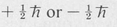
The total angular momentum of an electron in an atom then consists of the vector sum of its orbital angular momentum I and its spin s. The total angular momentum of a single electron, denoted by the symbol j, is then given by

(8.49)

It is customary to express the various angular momenta in units of ħ. The angular momenta in these units are then essentially quantum numbers. For a given value of the azimuthal quantum number /, there are two values of the quantum number for the total angular momentum of a single electron, namely,

(8.50)

Thus for l = 1, j = 3/2 or 1/2, for / = 2, j = 5/2 or 3/2, and so forth. For the case / = 0 there is only one value because the two states j = + 1/2 and j =– 1/2 are actually the same.

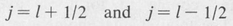
Now it was stated earlier that those states of hydrogen with a given value of the principal quantum number n, all have the same energy. This is not strictly true since the electron spin was not taken into account. Actually, as the electron undergoes its orbital motion around the positively charged nucleus, it experiences a magnetic field arising from this motion. The magnetic moment associated with the spin interacts with the magnetic field. This is called spin-orbit interaction. 19 The result of the spin-orbit interaction is that the two states j = l + s and j = l–s have slightly different energies. This in turn produces a splitting of the spectrum lines. A simplified diagram illustrating the splitting for the case of a p → s transition is shown in Figure 8.12.

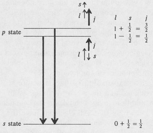
Figure 8.12. Fine structure (spin splitting) of a spectrum line for a p → s transition.

8.8 Multiplicity in the Spectra of Many-Electron Atoms. Spectroscopic Notation

For atoms containing more than one electron, the total angular momentum J is given by the vector sum of all the individual orbital momenta I₁, I₂, . . . , and spins s₁, s₂, . . . , and so forth.

In the usual case the orbital angular momenta couple together to produce a resultant orbital angular momentum L = I₁ + I₂ + .... Similarly, the spins couple to form an overall resultant spin S = s₁ + s₂ + .... The total angular momentum is then given by the coupling of L and S,

(8.51)

This type of coupling is known as “LS coupling.” Other types of coupling can also occur, such as “jj coupling” in which the individual js add together to produce a resultant J. In general, LS coupling occurs in the lighter elements and jj coupling in the heavy elements.

In LS coupling all three quantities L, S, and J are quantized. Their magnitudes are given by

where L, S, and J are quantum numbers with the following properties.

The quantum number L is always a positive integer, or zero. The spin quantum number S is either integral or half integral, depending on whether the number of electrons is even or odd, respectively. Consequently, the total angular-momentum quantum number J is integral, or half integral, depending on whether there is an even or odd number of electrons, respectively.

The total energy of a given state depends on the way the various angular momenta add together to produce the resultant total angular momentum. Hence, for given values of L and S the various values of J correspond to different energies. This in turn results in the fine structure of the spectral lines.

The spectroscopic designation of a state having given values of L, S, and J is the following:

^2S+1L_J

Here the quantity 2S + 1 is known as the multiplicity. It is the number of different values that J can assume for a given value of L, provided L ≫S, namely,

L + S, L + S–1, L + S–2, . . . L–S

If L < S, then there are only 2L + 1 different J values, namely,

L + S, L + S–1, L + S–2, . . . ∣L–S ∣

This is known as “incomplete multiplicity.”

If S = 0, the multiplicity is unity. The state is then said to be a “singlet.” Similarly, for S = , the multiplicity is two, and the state is a doublet. Table 8.3 lists the spin, multiplicity, and names of the first few types of states.

For one-electron atoms, only one value of S is possible, namely, . Hence all states of one-electron atoms are doublet states. In the case of two electrons, S can have either of the two values = 1 or = 0. Thus for two-electron atoms there are two sets of states, triplets and singlets.

In addition to the naming of states according to multiplicity, a letter is used to designate the value of the total orbital angular momentum L. This designation is given in Table 8.4.

The letter S, designating states for L = 0, is not the spin quantum number, although it is the same letter. This is confusing, but it is accepted convention.

Table 8.3. MULTIPLICITIES OF STATES

————————S————Multiciplity (2S + 1)—————Name—————————
0	1	Singlet
	2	Doublet
1	3	Triplet
	4	Quartet
2	5	Quintet
	6	Sextet

Let us consider, as an example, the case of two electrons. Let one electron be a p electron (l₁ = 1 ) and the other be a d electron (l₂ = 2). The possible values of L are l₁ + l₂, ∣l₁–l₂∣, and all integral values between. Thus L = 1, 2, or 3, which means that we have P states, D states, and F states. Since S can be 0 or 1, then there are both singlets and triplets for each L value. The complete list of possible states for the combination of a p and a d electron is the following:

Selection Rules In the case of LS coupling, the selection rules that govern allowed transition for dipole radiation are the following:

ΔL = 0, ± 1
ΔS = 0
ΔJ = 0, ± 1 (J = 0 → J = 0 forbidden)

Table 8.4. DESIGNATION OF STATES ACCORDING TO ORBITAL ANGULAR MOMENTUM

In all cases the symbol Δ means the difference between the corresponding quantum numbers of the initial and final states of the transition.

Parity In addition to the above selection rules there is another important rule involving a concept known as parity. The parity of an atomic state can be even or odd. This is determined by the sum of the / values of the individual electrons. If the sum is even (odd), the parity is even (odd). For example, consider the states of a two-electron atom. If one electron is an s electron (l₁ = 0) and the other is a p electron (l₂ = 1), then l₁ + l₂ = 1, hence all sp states are of odd parity. Similarly, all sd states are of even parity, and so forth. The following selection rule holds for electric dipole radiation from transitions between two states:

In other words the parity of the final state must be different from the parity of the initial state.

It is possible for an excited state to be such that it cannot undergo a transition by dipole radiation to any lower state. In this case the state is said to be metastable. If an atom is in a metastable state, it must return to the ground state either by emission of radiation other than dipole radiation–for example, quadrupole, and so forth–or it may return via collisions with other atoms.

8.9 Molecular Spectra

Molecules, like atoms, are found to exhibit discrete frequency spectra when appropriately excited in the vapor state. This indicates that the energy states of molecules are quantized and that a molecule may emit or absorb a photon upon changing from one energy state to another.

For purposes of spectroscopy, the energy of a molecule may be expressed as the sum of three kinds of energy. These are rotational energy E_rot, vibrational energy E_vib, and electronic energy E_el. Thus

E = E_rot + E_vib + E_el

Of the three, E_rot is generally the smallest, typically a few hundredths of an electron volt. Vibrational energies are of the order of tenths of an electron volt, whereas the largest energies are of the electronic type that are generally a few electron volts. Each of the three types of energy is quantized in a different way and, accordingly, each is associated with a different set of quantum numbers.

It is possible for transitions to take place that involve the rotational energy levels only. The resulting spectrum, called the pure rotation spectrum, usually lies in the far infrared or the microwave region. If vibrational changes also occur in the transition but no electronic changes, we have the rotation–vibration spectrum. The rotation–vibration lines are generally found in the near infrared. Finally, transitions that involve electronic-energy changes are the most energetic. Lines of the electronic spectra of molecules occur typically in the visible and ultraviolet regions.

Rotational Energy Levels The rotational energy, E_rot, is the kinetic energy of rotation of the molecule as a whole. The quantization of the rotational energy is expressed in terms of rotational quantum numbers. How many of these rotational quantum numbers are needed to specify a given rotational state depends on the particular molecular geometry. There are four basic molecular types. These are

1. Linear molecules
2. Spherical-top molecules
3. Symmetrical-top molecules
4. Asymmetrical-top molecules

The four types are illustrated in Figure 8.13.

In the case of linear molecules and spherical-top molecules, only one quantum number J is needed to specify the rotational state. As with atomic states, the quantity is the magnitude of the rotational angular momentum. The rotational energy is given by the quantum equivalent of the classical value, namely,

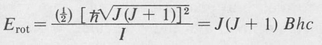
(8.52)

where

(8.53)

and

J = 0, 1, 2, . . .

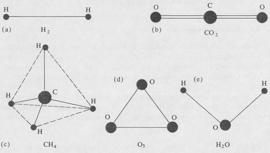
Figure 8.13. Some cases to illustrate the different types of molecular rotational symmetry. (a), (b) Linear molecules: I_a = I_b, I_c = 0; (c) spherical top: I_a = I_b = I_c; (d) symmetrical top: I_a = I_b ≠ I_c; (e) asymetrical top: I_a ≠ I_b ≠ I_c.

Here I is the moment of inertia of the molecule about the axis of rotation. (For a symmetrical diatomic molecule consisting of two atoms of mass M/2 separated by a distance 2b, the moment of inertia is given by the classical expression I = Mb².) An energy-level diagram showing the rotational levels of a linear molecule is shown in Figure 8.14.

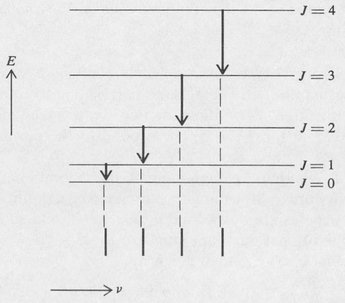
Figure 8.14. Transition diagram for a pure rotational spectrum.

In the case of symmetrical-top molecules, two quantum numbers are needed to specify the rotational states. These are customarily written as J and K, where, again, is the total rotational angular momentum. The quantum number K is the component in units of ħ of the rotational angular momentum about the symmetry axis. For a given value of K, J can assume any of the values K, K + 1, K + 2, and so forth. The rotational energy levels are then given by the formula

(8.54)

In the above formula the quantities B and C are related to the two principal moments of inertia of the molecule,

(8.55)

Here I_c is the moment of inertia about the symmetry axis, and I_b is the moment about the perpendicular axis.

In the case of the asymmetrical-top molecule, there are three different moments of inertia, and three rotational quantum numbers are involved. The theory is quite complicated in this case, and there is no simple formula for the energies of the quantized states [23].

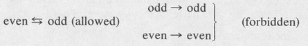
Rotational transition rules are governed by the general selection rules

(8.56)

In addition to the above rules, there are other selection rules involving the symmetry of the rotational states. We shall not go into a discussion of these.

Vibrational Energy Levels If a molecule contains N atoms, there are 3N modes of motion. Of these, three correspond to translation of the molecule, and three to rotation (or two for a linear molecule). The remaining 3N — 6 (or 3N — 5) correspond to the normal vibrational modes.

Theory shows that the quantizing of each vibrational mode can be expressed in terms of a single associated quantum number. The normal frequencies are designated v₁, v₂, . . . , and so forth, and the associated vibrational quantum numbers are v₁, v₂, . . . , and so on. The vibrational energy is then given by

(8.57)

The above formula is valid if the vibrational displacements are small enough so that the motion is essentially harmonic in character. It indicates that the energy levels associated with a given normal mode are (1) equally spaced, and (2) the energy of the lowest vibrational state (v₁ = 0, v₂ = 0, ...) is not zero, but has a finite value: . . . . This energy is called the zero-point energy. It is present even at the absolute zero of temperature.

The selection rule for vibration transitions is

(8.58)

This rule is strictly adhered to only if the motion is absolutely harmonic. Such is never actually the case. Transitions in which Δv = ± 2, ± 3, and so forth, also occur. These overtone transitions are generally much weaker than the fundamental transitions in which Δv = ± 1.

A homonuclear diatomic molecule does not exhibit a pure rotation spectrum nor does it show a rotation-vibration spectrum. This is because homonuclear molecules have no permanent electric dipole moment. Consequently neither rotational nor vibrational transitions produce an oscillating dipole moment. Thus there is no associated dipole radiation.

On the other hand heteronuclear diatomic molecules such as hydrogen chloride do exhibit strong rotation-vibration spectra.

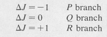
A transition diagram illustrating the vibrational energy levels of a diatomic molecule, with rotational energy levels superimposed, is shown in Figure 8.15. The J-selection rule for rotation-vibration transitions is

(8.59)

The spectrum is divided into three branches known as the P, Q, and R branches. They are determined by the value of ΔJ as follows:

Electronic Energy States in Molecules The following discussion is restricted largely to the case of diatomic molecules, although many of the general principles apply to other molecules as well.

In molecules, the orbital angular momenta and spins of the electrons couple together in much the same manner that they do in atoms. In diatomic molecules, an important quantum number is one designating the sum of the projections of the orbital angular momenta on the line connecting the two atoms. This quantum number is denoted by the symbol Λ. The various electronic states corresponding to different values of Λ are designated by capital Greek letters as follows:

Λ : 0, 1, 2, 3, ...

Electronic state : Σ, Π, Δ, Φ, . . . .

For a given value of Λ, the rotational quantum number J can have any of the values Λ, Λ + 1, Λ + 2, and so forth.

As in the case of atoms, the total spin S determines the multiplicity of an electronic state. This multiplicity is 2S + 1. It is the number of sublevels for a given value of J. Thus there are singlet

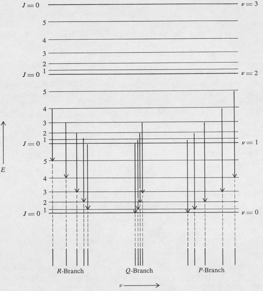
Figure 8.15. Transitional diagram for a rotation-vibration spectrum.

states (S = 0):

¹∑, ¹∏, ¹∆, ...

doublet states (S = 1/2):

²∑, ²∏, ²∆ ...

and so on. It is also true, as with atoms, that the multiplicity is always odd (even) if the total number of electrons is even (odd).

The selection rules governing electronic transitions are

(8.60)

(8.61)

The following are examples of allowed electronic transitions:

¹∑ → ¹∏, ²∏ → ²∆ ³∏ → ³∑

Since the electronic energies in molecules have the rotational and vibrational energies superimposed on them, electronic transitions may be accompanied by vibrational and rotational transitions. This results in a very large number of lines for each electronic transition and gives rise to the vibration-rotation structure in the electronic spectra of molecules. A partial energy-level diagram of the nitrogen molecule N₂ is shown in Figure 8.16 as an example.

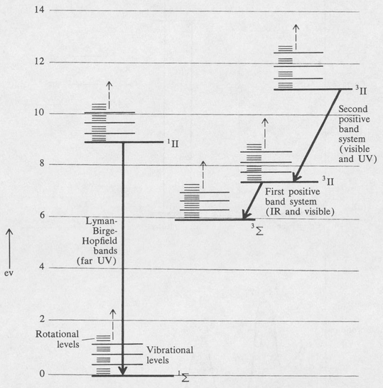
Figure 8.16. Partial energy-level diagram of the nitrogen molecule N₂. Electronic transitions of some of the important band systems are indicated. The rotational and vibrational energy levels are not drawn to scale.

8.10 Atomic Energy Levels in Solids

Consider an atom that is embedded in a solid, either as a part of the structure or as an impurity. One or more of the electrons may be shared by the solid as a whole, and thus are not associated with any particular atom.

Figure 8.17. (a) Energy level diagram of the Cr³⁺ ion in the free state and in ruby; (b) absorption of the Cr³⁺ ion in ruby.

The energy levels of these electrons become smeared out into bands—the valence and conduction bands—of the solid. The atom in question then becomes an ion. The bound electrons associated with the ion may have various quantized states available to them and therefore various energy levels. This gives rise to a characteristic ionic absorption spectrum.

In the case of the rare earth ions, the unfilled shells involve deep-lying 4f electrons. These electrons are well shielded by the outer electrons, and the energy levels of the free ion are essentially unchanged when the ion is embedded in a solid. The levels are quantized according to angular momentum and are designated in the same way as the regular atomic energy levels discussed in Section 8.2.

For the transition metals, such as iron, chromium, and so forth, the 3 d shell is unfilled. This shell is not as well shielded as the 4f shell in the rare earths. The result is that the energy levels of transition metal ions are profoundly changed when the ion is placed in a solid. Rather than angular momentum, it is the symmetry of the wave function that is important in the determination of the energy levels in this case, particularly if the ion is in a crystal lattice. The quantization of the energy is then largely dictated by the symmetry of the field due to the surrounding ions.

It is beyond the scope of this book to develop the theory of atomic energy levels in crystals. The subject is very involved. An extensive, rapidly growing literature already exists. However, as an illustration of the energy-level scheme of a typical case, the levels of the Cr³⁺ ion are shown in Figure 8.17. At the left are shown the levels of the free ion, while at the right are the levels of the Cr³⁺ ion in ruby. The symbols A, E, and T refer to different types of symmetry. The ruby crystal consists of Al₂O₃ (corundum) in which part of the aluminum atoms have been replaced with chromium. The red color of ruby is due to the absorption of green and blue light corresponding to transitions from the ground state, ⁴A, to the excited states ⁴T₁ and ⁴T₂, as indicated.

For further reading in atomic, molecular, and solid-state spectroscopy, References [18] [19] [23] [24] [30] and [40] are recommended.

PROBLEMS

• 8.1 If R is the Rydberg constant for a nucleus of infinite mass, Equation (8.9), show that the Rydberg constant for a nucleus of mass M is given approximately by R_M ≈ R — (m/M)R.
• 8.2 Calculate the difference between the frequencies of the Balmer — α lines of hydrogen and deuterium.
• 8.3 Calculate the frequency of the hydrogen transition n = 101→ n = 100.
• 8.4 Show that the energy of the 2s state of atomic hydrogen (Table 8.2) is R by substitution in the radial Schrödinger equation (8.36).
• 8.5 Consider a hydrogen atom in the ground state and imagine a sphere of radius r centered at the nucleus. Derive a formula for the probability that the electron is located inside the sphere. (a) What is the probability for r = a_H? (b) For what value of r is the probability equal to 99 percent?
• 8.6 Determine all of the states of a pf configuration of two electrons in LS coupling.
• 8.7 Find all of the allowed dipole transitions between a pd and a pf configuration.
• 8.8 Calculate the lifetime of the 2p state of atomic hydrogen by assuming that the magnitude of the dipole moment of the transition to the 1 s state is approximately equal to ea_H.
• 8.9 Find the frequency of the radiation emitted by the pure rotational transition J = 1 → J = 0 in hydrogen chloride. The distance between the hydrogen atom and the chloride atom is 1.3 A.