FIFTEEN
WKB Near Caustics
From our work on the WKB approximation it is clear that an interesting sort of trouble can arise if the function f(t) of (14.33) vanishes at t = T or equivalently if ∂2S/∂a ∂b is infinite. In either the discrete (finite N) or the continuous case, this vanishing has been found to be due to the vanishing of one or more eigenvalues of δ2S(N) (or δ2S). For the quadratic Lagrangian we were stuck with this blowup. It meant that there was perfect focusing and the Green’s function became a δ-function. But now with δ3S terms available, the blowup occurs only in an approximation and in fact the Green’s function remains finite.
Consider, then, values a, b, and T such that one of the eigenvalues of δ2S along a particular classical path vanishes. Thus b at time T is a conjugate point for the trajectory leaving a at time 0. Holding (a, 0) fixed, we consider the Green’s function in a neighborhood of b, G(b+Δb, T; a). Again we work with G(N), but we do not worry about distinguishing  , the exact trajectory connecting the conjugate points, and
  , the solution of the discrete problem—for which the vanishing eigenvalue may differ from zero by terms of O(ε).h Our expansion will differ from those we considered previously. Paths from (a, 0) to (b + Δb, T) will not be expanded about the classical path connecting those endpoints but rather about
  This means that the variational path does not vanish at the upper limit, and we have some extra terms to carry along. Next define the path ρ(t) to be some fixed arbitrary curve with ρ(0) = 0, ρ(T) = Δb; ρ can be chosen in some convenient way, but for our purposes it is left arbitrary. The path x(τ), the “integration variable” of the path integral, is written

(15.1)
so that y(0) = 0, y(T)=0. As usual by a translation the new integration variable is y(τ), and again we expand
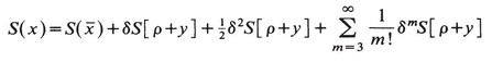
(15.2)
Now, however, δS does not vanish; in particular
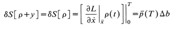
(15.3)
 is the momentum of
  at T and for n dimensions it is the vector dot product that appears in (15.3). The second variation is

(15.4)
(see (14.9) for the definition of W).
The quantity δ2S [ρ] is some fixed number which we ignore for now. In the cross term of (15.4) we do an integration by parts to obtain
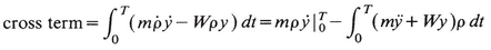
(15.5)
The function y has the same boundary conditions as the Sturm-Liouville eigenfunctions (see discussion at (12.9)—(12.11)) and can be expanded in terms of them:

(15.6)
Call the eigenvalues λ1, λ2,.., with λ1 <λ2<  . Again we have

(15.7)
but now λ1 = 0, because we are at a conjugate point. Thus  does not appear in δ2S. Equation 15.5 can also be rewritten, and becomes
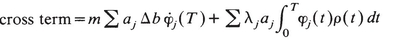
(15.8)
We next change variables to {ai} instead of {y¡} but ignore details of the Jacobian, which would have been calculable had we been strict in remembering that we are dealing with G(N). We have obtained therefore the following form for the Green’s function:
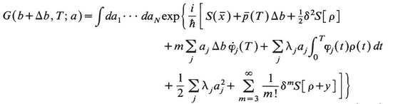
(15.9)
What is new and interesting about this integral is the absence of an  term in the exponent so that for Δb = 0 the leading term in a1 is cubic. However, to see the consequences of this feature a good deal of underbrush must be cleared away, namely the other N—1 integrals over a2,..., aN. We do this in two ways: one, by using previous experience with asymptotic limits to assign powers of
  to various contributions and then noting that everything works out self consistently. We apply this method only for Δb small. The second way appeals to some theorems from the general body of knowledge known as catastrophe theory to obtain a normal form for the integrand for which the limitation to small Δb can be lifted so as to obtain a “uniform asymptotic approximation.” That is done in Section 16.
In our first approach to the integral (15.9) we look upon the argument of the exponent as a power series in the a’s. In previous sections we discarded terms of 0(aiajak)/ as being O(3/2/)=O(1/2) relative to the leading quadratic term. Now, with  missing, the procedure must be reexamined.
First let us estimate the size of a1. Consider an integral of the form

By rescaling, this becomes (assuming that the limits of integration are unimportant) 
so that each power of x contributes µ-1/3. This suggests that for →0 a1 is O(1/3). Next consider Δb and ρ. By its definition, ρ can be selected so that O(ρ) = O(Δb). Δb is an external parameter and is at our disposal. Since we are only seeking a description of the Green’s function in the critical region, it is enough to consider Δb such that a1Δb=0(). This is because the principal a1 contributions to the integral are from  and a1Δb. When these are of the same order the character of the integral is no longer dominated by the cubic (in fact, it can be rewritten as a quadratic with coefficient ∼(Δb)1/2). Hence the critical region—where G is most singular—is characterized by
  and we restrict our attention to this domain.
Terms  for j≠1 are the usual quadratic terms which will ultimately dominate the integrals ∫daj, j≠1. We therefore assume that we can proceed in the ordinary way and take aj=0(1/2), j≠1.
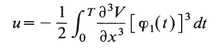
Next we must estimate the linear terms in aj, j≠1 and higher-order terms involving all aj’s that appear in δkS, k≥3, Linear terms ajΔb and aj∫ϕρdt, j≠1 , are unimportant to leading order in since aj=O(1/2) and Δb=O(2/3). Hence this is smaller by 1/6 than the quadratic term  which gives the dominant contribution. Of the higher-order terms we consider only the third variation, which is

(15.10)
and which includes terms in the following 10 categories:
| I. |  |
|
| II. |  |
j≠ 1 |
| III. | a1ajak | j, k≠ 1 |
| IV. | ajakan | j, k, n≠1 |
| V. |  |
|
| VI. | a1aj∫p | j≠1 |
| VII. | ajak∫ρ | jk≠1 |
| VIII. | a1(∫ρ)2 | |
| IX. | aj(∫ρ)2 | j≠1 |
| X. | (∫ρ)3 |
The term  is of course the important contribution for the a1, integral. By our previous estimate it is O(
 ). By going through the rest of the list it is immediately evident that all other terms are O(7/6) or smaller. It is also clear that the worst terms in δkS, k ≥ 4, are O(4/3) and so need not be considered.
To leading order in the Green’s function is therefore

(15.11)
with
(15.12)

(15.13)
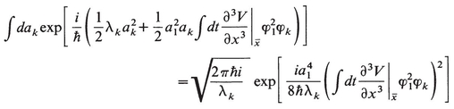
The integrals over aj, j ≠ 1 will as usual give (Π′λj)—1/2, the prime over II denoting that the term j= 1 is excluded. Recalling that the product over all λj gives a quantity f(T) related to a certain solution of the Jacobi equation [cf. Section 6 or (14.32) and 14.33)], we write Π′λj=f(T)/λ1. Although for the conjugate point both f(T) and λ1 vanish, the ratio is finite. In fact it is just by looking at that ratio that one can sometimes compute Π′λj. (Such a calculation occurs in Section 29 in connection with “instantons.”)
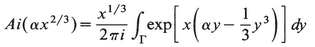
There remains only the integral over the cubic polynomial. Recall the definition of the Airy function
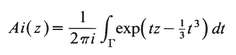
(15.14)
with the contour Γ shown in Fig. 15.1. This can also be written as

(15.14a)
Some properties of the Airy function are


Fig. 15.1 Contour Γ in the complex t plane for evaluating the Airy function (15.14). Γ goes to infinity asymptotically in the left half plane and at angles exceeding π/6 to the negative real t axis.
(J is the Bessel function). For real z

(15.15)
It follows that the cubic integral is just an Airy function, and by comparing (15.11) and (15.14) we note that G contains the factor Ai(υu—1/3—2/3). One cosmetic step remains before giving our final form of G. The quantity  is the momentum along
  at the time T and is therefore equal to
  . Therefore
S( ) +
) +  (T)Δb= S(class. path a→b + Δb)≡Sc(b + Δb, T; a)
The Green’s function to leading order in is
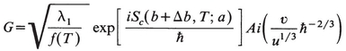
(15.16)
(leaving out factors π, etc.).
The expression (15.16) does not differ by much from that which we derived in Section 16 without the restriction Δb  2/3 (and therefore υ
  2/3). Hence we examine (15.16) for qualitative information on G. The limit →0 corresponds to |z| [of (15.14)] going to infinity. Consequently (15.15) suggests that the behavior of G (in the limit →0) depends strongly on the sign of υ/u1/3. For υ/u1/3 > 0 the Green’s function has an exponential decay—going to zero as exp[-(Δb)3/2·const.]—while for υ, having the opposite sign, G has a sinusoidal dependence. The changing sign of υ/u1/3 is just that of Δb [cf. (15.13)] as one goes through the conjugate point. Thus one side of the conjugate point is in “shadow.” The Green’s function, hence the probability of the system’s being there is small. On the other side is “illumination,” that is, high probability of finding the system. The “brightest” region is just near the conjugate point. There the asymptotic expansions for the Airy functions cannot be used. For example, at
  =b(Δb=0)

(15.17)
This is large, since the typical contribution of each degree of freedom to G is of order 1/2 rather than 1/3. Thus within the critical region of the conjugate point there is a greater propensity for nonclassical effects reflected in the appearance of lower powers of .
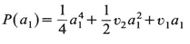
We have given arguments in one space dimension. In higher dimension “υ” depends on
where ϕ1(t) is the solution of the appropriate vector Jacobi equation. In general, there will be a surface of conjugate points; on one side of the surface will be “illumination” and on the other side shadow. Such a surface in optics is known as caustic (see Fig. 15.2). We shall have more to say below about caustics, as well as their relation to catastrophes, but for now let us consider (15.16) a bit more closely.
The phenomenon revealed by G of (15.16), the passage from a high probability region to a low probability region as one crosses the conjugate point, does not present a new mystery, but rather solves an old problem that we have swept under the rug again and again in the course of this work. In using the semiclassical approximation we have always required the classical paths (solutions of the Euler-Lagrange equations) to be well separated from one another. The Green’s function we have just derived is precisely that appropriate for the case of two coalescing classical paths.
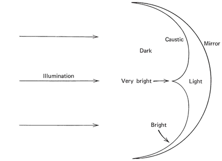
Fig. 15.2 A commonly observed caustic—one that arises from a cylindrical mirror with circular cross section. This is often seen on the surface of a cup of coffee under appropriate conditions of illumination.
First a heuristic justification of the statement above: we digress a bit, to say what problem the Airy function solves. By a change of variable we can write
(15.18)
with x>0. For fixed α and large x one of the two forms of (15.15) is obtained. These two forms arise because when one uses steepest descent methods for (15.18) he encounters the equation

For α>0 this has no solution on Γ (cf. Fig. 15.1) while for α<0 there are two solutions. For α<0 one therefore obtains the larger values of Ai while for α<0 the integral has only an exponentially small term arising from a critical point off the range of integration. If α is allowed to vary, and in particular if it can be small on the order of x—2/3, then all bets are off. The asymptotic approximations do not give useful results, and the best that one can say is “it’s an Airy function.” The trouble of course arises because of the coalescing of the two critical points y=  . For α small their contributions interfere (so the asymptotic approximation which writes Ai as a sum of two distinct terms is inaccurate) while for the wrong sign of α, although the appropriate value of y does not appear on Γ, it is not far away.
For the path integral it is zeros of δS that are the critical points and for the given initial point and the given T the classical mechanics (boundary value problem) has two solutions on one side of the conjugate point and none on the other. To see this rigorously, observe that the argument of the exponent in (15.9) is just the classical action, expressed in rather peculiar coordinates, the variables aj, j=1,..., N. The quantities  ϕj, and so on, are fixed, and the problem of finding a solution to δS=0 is the same as requiring that ∂/∂aj vanish for each j. For j≠1 there is always a solution because the derivative of the leading quadratic term
  gives a linear equation for aj which has a solution near zero (for small Δb). For a1, referring to (15.11), the equation is
  =0 which may have zero or two solutions depending on the sign of υ/u (υ≠0). This justifies the description of the phenomenon in (15.16) as the coalescing of classical paths.
There is an obvious generalization of the results obtained so far. Suppose there is a region in coordinate space where u of (15.12) vanishes along with λ1 so that the leading term in a1 is  . Then the propagator can be brought to the form
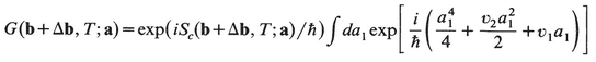
(15.19)
with υ1 and υ2 dependent on Δb and vanishing when Δb=0. The point b is even more brightly illuminated than in previous cases. Moreover, in some directions out of the point b the polynomial
(15.20)
has points where it is stationary and also its second derivative vanishes. This means that by a shift in variable we are again on a caustic but one of lower order, one in which a cubic polynomial determines the behavior. The equation of this caustic is obtained by finding those (υ1, υ2) for which the equations dP/da1=  = 0 can be solved simultaneously. The required relation between υ1 and υ2 is

(15.21)
which is a cusp. The quantities υ1 and υ2 are definite calculated functions of Δb, υ1 being a coordinate in the direction  , and υ2 a coordinate in a perpendicular direction. Thus this particular caustic assumes a specific form, that of the cusp. See the “very bright” point and its neighborhood in Fig. 15.2.
Suppose that at some b, both λ1 and λ2 are zero. G will then involve a double integral, and it is obvious that terms in a1 and a2 will appear with coefficients related to  and
and  . But this is not all. The component of Δb along the direction
 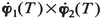 will also control the development of the caustic due to terms from δ3S. The propagator can therefore be written

(15.22)
where P can be brought to the form
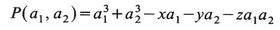
(15.23)
We can in this way obtain an entire class of functions giving a description of the wave function near a caustic. Those of the kind presented in (15.20) have been given the name “generalized Airy functions,” and it would seem that the propagator of (15.22) with a polynomial in several variables would warrant such a designation also.
The picture that emerges is that a certain polynomial [e.g., (15.23)] by virtue of its appearing in an integral with a large parameter governs the form taken by the caustic. Specifically, several of the coefficients of the lower powers in the polynomial are functions of position. The location of the caustic corresponds to the values of the coefficients for which the polynomial has simultaneously vanishing first and second derivatives.
To anyone exposed to catastrophe theory these results declare in no uncertain terms that caustics are catastrophes. To go into an exposition of catastrophe theory at this point would be too great a digression, so our next few remarks will have to be obscure to those unfamiliar with the subject. (In this we shall be loyal to the traditions of catastrophe theory: it always sounds like a snow job.)
The foregoing work has in effect been an explicit example of the successful operation of the principles of catastrophe theory, namely morphology has been determined by a breakdown in structural stability. The caustics are located by finding those values of the coefficients of the polynomials P for which P, considered as a potential, is not structurally stable. Moreover the theory provides us with a map from the space of coefficients to physical coordinate space. The form of the caustic is not sensitive to the details of this map, and so for example the cusp of (15.21) may be expected to be a common sort of caustic: not in its detailed global behavior but in its form near the singularity.
The present development is also an object lesson in the limitations of catastrophe theory. Although the loci of breakdown in structural stability (which is all catastrophe theory can give you) are correctly obtained, the details of the propagator (e.g., how much brighter is the caustic region than other regions) can only be obtained by looking at the underlying theory (in this case quantum mechanics) governing the phenomenon.
In the next section we turn to the problem of obtaining the propagator at larger distances from the caustic, that is, relaxing the condition  and finding “uniform” approximations. Oddly enough I believe that here an important mathematical role is played by one of the theorems used in catastrophe theory, but not the much publicized classification of the “seven elementary catastrophes.”
NOTES
Section 15 is an expansion of parts of the following paper
L. S. Schulman, Caustics and Multivaluedness: Two Results of Adding Path Amplitudes, in Functional Integration and Its Applications, Proceedings of a 1974 conference, A. M. Arthurs, Ed., Oxford University Press, London, 1975
As mentioned there, parts of that work were in turn based on the dissertations of Steve Coyne and David McLaughlin:
S. Coyne, Semi-Classical Asymptotic Evaluation of Feynman Path Integrals, thesis, Indiana University, Bloomington, Ind., 1972
D. W. McLaughlin, The Path Integral: Its Approximation in Flat Space and its Representation in Curved Space, thesis, Indiana University, Bloomington, Ind., 1970
In obtaining the canonical form of a fourth-order caustic, (15.19), we ignored a subtlety that did not occur for the third-order caustic. For third-order caustics we went through a list of terms that appear in the action [just following (15.10)] and determined that only the term involving  need be considered. A similar list for a fourth-order caustic would include terms
  ak(k = 2, 3, ...) in the action. These are of order , the same as
  , and cannot be dropped. However, these terms do not affect the validity of (15.19), and if no convergence problems erupt they simply serve to change the coefficient of the quartic term. To see this, consider what happens to such a term when the integral over ak(k≠ 1) is performed
Consequently the coefficient of  is
is
rather than merely the first term alone. To get the form of (15.19) one must in any case perform a rescaling of a1 and provided the above mentioned sum exists this can be done.
For caustics of yet higher order the same sort of thing is feasible. What is important is that one should never get terms of the form  to be significant, for then one could not perform the integrals dam, m > 1 one at at a time to eliminate such terms. But both aj and ak are O(1/2) and so this problem cannot develop.
The argument just given for the  terms going over to
  terms makes no pretense of rigor and as often happens in asymptotic analysis the desired result is best obtained by the use of the implicit function theorem. The coordinate system that we use for integration was gotten from the diagonalization of δ2S, whereas for the elimination of the cross terms a slightly different coordinate system would be best. The existence of such a coordinate system is shown in
R. S. Ellis and J. S. Rosen, Asymptotic Expansions of Gaussian Integrals, Bull. Amer. Math. Soc., 3, 705, 1980
Ellis and Rosen were looking at the Wiener integral and were able to extend rigorous results on the asymptotic expansion of the Wiener integral (see the Schilder reference in Section 14) to the case of degenerate and coalescing minima. Because they looked at the real Wiener integral they never had the privilege of treating the “easy” cubic case and used the implicit function theorem to show that at degenerate critical points the measure picks up a non Gaussian part, like our  term.
term.
The derivation of the caustic-catastrophe connection through path integration has proved to be an attractive method, and further work on this theme has been done by
Cecile DeWitt-Morette and P. Tschumi, Catastrophes in Lagrangian Systems, in Long Time Predictions in Dynamics, ed. V. Szebehely and B. D. Tapley, Reidel, Dordrecht, Holland, 1976, pp. 57—69
Cecile DeWitt-Morette, The Semiclassical Expansion, Ann. Phys. 97, 367 (1976)
S. Levit, U. Smilansky, and D. Pelte, A New Semiclassical Theory for Multiple Coulomb Excitation, Phys. Lett. 53B, 39 (1974)
A good expository article on catastrophe theory, containing many references, is
M. Golubitsky, An Introduction to Catastrophe Theory and its Applications, SIAM Review 20, 352 (1978)