Cell Basics

You’ll be spending lots of time selecting cells and moving around in tables, so knowing how to select and Move between Cells will save you lots of time; you’ll find most options are relatively intuitive even if you haven’t worked in a spreadsheet before.

This chapter also covers how to Merge and Unmerge Cells, and what happens to the data in them when you do either. (Formatting cells is covered in separate chapter, cleverly named Cell Formats.)

Cell Referencing 101

You’ve probably already realized that a single cell is named, Bingo-like, for its column and row: B2, E6, and so on.

Multiple cells in a group (referred to variously as a block, range, array, or collection) are named for the top-left and bottom-right cells, with a colon between: A2:A6 or B5:D10, for instance. (As detailed later, in Cell References, cells and cell groupings—and even cells in other tables—can be described in many ways inside formulas.)

Select Cells

To select a cell, just click it. Once the cell is selected, it’s ready for action: type something and it goes in the cell; press Delete and the cell contents disappear.

In true Mac fashion, you can select multiple cells by dragging across them, and you can add non-contiguous cells to a selection by Command-clicking each one. (Options for selecting whole rows and columns are covered earlier, in Select Rows and Columns.)

When a cell or group of cells is selected, the blue frame surrounding the selection has white circles, called selection handles, at its upper-left and lower-right corners; drag either one to change the selection, enlarging or shrinking it.

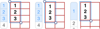
You can also extend a selection with a Shift-click in another cell, but what you wind up with depends on where you started. When you select a block of cells by dragging, the cell you first click in is the parent cell, and everything is calculated from there. Drag-select the block A1:A3 by starting in A1, then Shift-click in A4, and you wind up with A1:A4 selected. No problem, because that’s what you expected—but what you don’t realize is that the Shift-click is selecting all the cells from the parent cell to the Shift-click spot. Start with selecting A1:A3 by dragging upward from A3, Shift-click in A4, and only A3:A4 is selected, as shown in Figure 20.

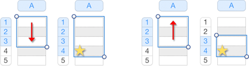
Figure 20: Adding to a selection with a click (marked by the star). Left: The initial selection is a drag from A1 to A3 so A1 is the parent. Right: The initial selection going from A3 to A1 makes A3 the parent.

You can also expand a selection by adding Shift to any keyboard option that moves you from one cell to another (except for Tab and Return, which reverse direction when you add the Shift key). So with the selection A1:A3 made by dragging from A1 to A3:

• Pressing Shift-Down arrow adds A4.
• Pressing Shift-Right arrow adds B1:B3.
• Pressing Command-Shift-Right arrow selects to the ends of rows 1, 2, and 3.
• Pressing Command-Shift-Down arrow selects to the end of column A.

Move between Cells

Since spreadsheets were invented (and the Mac keyboard added arrow keys) the four basic ways to move between cells have remained the same, and a few others have been added. To move:

• To any cell: Click in the cell.
• One cell down or up: Press Return to move down, and Shift-Return to move up.
• One cell right or left: Press Tab to move to the next cell, and Shift-Tab to move to the previous one.
• One cell in any direction: Use an arrow key.
• To the beginning or end of a row or column: Press Command along with an arrow key to jump from the current cell to the nethermost spot in any direction.
• To the first or last cell in a table: On a full keyboard, press Home to jump to A1 or End to go the last (lower-right) cell.

  On a laptop keyboard, it’s a two-step process. To jump to the first cell in the table, press Command-Up arrow to move to the first row; keep the Command key down and press Left arrow. The opposite—Command-Down arrow, followed by Command-Right arrow—gets you to the last cell.

When You Reach the End…

Tab and Return move you to the next cell—but what if there isn’t any “next” cell? If you’re at the end of a row (in the last column) and press Tab, you get a new column. Pressing Return when you’re at the bottom of the table creates a new row. (Logically enough, if you’re in a footer row, you get another footer row, but if you’re in the last body row above a footer, you’ll get another body row.)

If you’ve just typed data into the last cell of a column or row, it takes two presses of Tab or Return to add to the table: the first enters the new information in the cell, and the second adds the row or column.

When you’ve selected multiple cells, what happens when you move around by keyboard is dictated by the parent cell—the first place you clicked when you made the multiple selection. (That was described just above, in Select Cells)

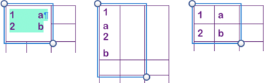
So, for instance, if you select the block A1:A4 by dragging from A1, pressing Tab or Right arrow moves you a single cell to the right of the parent cell, to B1. But if you select the block A1:A4 “backward,” by starting at A4, pressing Tab or Right arrow moves you out of the block, to B4—again, to the right of the parent cell (Figure 21).

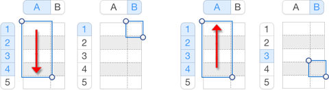
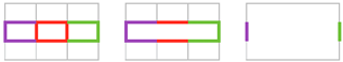
Figure 21: Left: Select starting from A1, and a subsequent Tab moves you to B1 (to the right of the parent cell). Right: Start the same selection from A4, and a Tab moves you to B4 (still to right of the parent cell).

You can take advantage of the parent cell concept to move within a small area with Tab and Return. Click in a cell, press Tab a few times to move a few cells, and then press Return: instead of going to the cell beneath the current one, you wind up in the one beneath the initial selection. Tab again to wherever, and when you press Return again, you move down a row in the parent cell’s column (Figure 22).

Figure 22: Click in a cell and it becomes a parent: press Tab to move right, and when you press Return, you wind up beneath the original, parent cell.

A click is not the only thing that makes a singly-selected cell a parent for this pattern: pressing Return makes any cell a new parent for tabbing and then Return-ing to the parent’s column.

Merge and Unmerge Cells

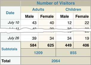
One of the most-used table-formatting procedures is also the easiest to accomplish: merging cells for headings, labels, or data that span multiple rows or columns, or for visually separating areas of a table (Figure 23). You can also merge cells that already contain data of any type, with varying consequences.

Figure 23: Cells can be merged horizontally or vertically, spanning as many rows or columns as needed. The blue text in this table is in merged cells.

Merging Basics

To merge cells, select them and choose Table > Merge Cells. To unmerge them (as you can probably guess), select the cell and choose Table > Unmerge Cells. Here are some simple guidelines:

• You can merge cells only if they live in the same area of the table: body, header, or footer.
• You can merge an already-merged cell with other cells; the Table menu command changes to Merge All Cells when you have such a group selected.
• You can’t merge cells if your selection includes hidden rows or columns; conversely, you can’t hide a row or column that contains a merged cell. You’ll find the related commands dimmed in these situations.

Merged Data

A merged cell retains the content of all its original cells. If only one cell in the merge group had data, the data remains as it was originally—it’s still text, a number, or a formula, for instance.

If more than one cell contained data, the data is combined with a tab separating each former column, and a paragraph return separating each former row. You can edit the merged data as needed. (If you mistakenly delete a tab separating data, type Option-Tab to replace it.)

Merged data is always treated as text, even if it was originally numbers, because of those tabs and returns. That means there are issues when formulas refer to an original cell or to the merged cell, as I detail just ahead.

Merged data isn’t always fully displayed in the merged cell; you may have to resize the cell to see all of it (Figure 24).

Figure 24: Left: The initial, separate cells. Right: Three examples showing seemingly different results of the merge depending on the sizing of cells.

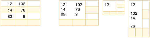
When you unmerge cells, the cells reappear in the table, but all the merged data remains in the upper-left cell of the unmerged group (Figure 25).

Figure 25: Left to right: Original cells selected; the merged cell; and the unmerged cells.

Merged Cells and Formulas

Merged cells can pose problems for formulas whether the cells contained formulas, or are referenced by formulas elsewhere:

• If a formula cell is the only one in a merged group that had anything in it, the formula is retained; otherwise, the result of the formula is included in the merged data.
• You can use only the top-left cell of a merged group as a reference in a formula. If, for instance, you’ve merged A2:A5, you can’t use A3 in a formula even though it’s part of the merged cell. Unless you use A2, you’ll get an error.
• If you use a cell range in a formula, it must include the entire range of the merged cell to avoid an error.
• If a formula references a cell that later becomes part of a merged cell, the formula may return an error, depending on the results of the merge. If the merged cell contains data that’s usable in the formula, you won’t get an error message (although you’ll likely get unintended results).

Redistributing Unmerged Data

So, you merged data from a block of cells and would like to get the data back into separate cells? It’s not obvious, but it’s easy:

1. Copy the contents of the merged cell before you unmerge it: double-click in the cell to activate the contents, and choose Edit > Select All, and then Edit > Copy.
2. Choose Table > Unmerge Cells.

   All the data is in the upper-left cell, even if you can see only the first piece of data, and all the cells that were originally merged are selected. (It’s not necessary to have all the cells selected for the next step to work; you can instead have only the upper-left cell of your target area selected.)

3. Choose Edit > Paste (Figure 26).

Figure 26: Left: The selected contents to be copied in a merged cell. Center: The unmerged cells. Right: Original contents restored by pasting into the unmerged cells.

This little trick works because multiple data items in the merged cell are separated by tab and return characters, as explained previously. And when you paste tab-delimited information into a table, the tabs separate the data into cells, and returns define rows.

Formats in Merged Cells

When you merge cells, it’s not just the data that gets combined: cell fill color, borders, text formatting, and data formatting are also affected.

Fill Color

Merged cells inherit their fill color from the first (top-left) cell in the group. When you unmerge them, the formatting remains in the first cell (as does any formatting you apply to the merged cell). The other cells revert to no background, even if they had color prior to the merge.

Borders

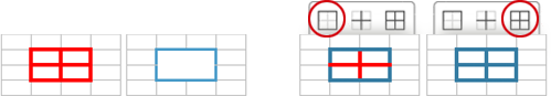
Borders for a merged cell are patchworked together from the borders used on the original cells (Figure 27). (Applying borders to cells is covered in Cell Borders.)

Figure 27: Left: Three bordered cells. Center: The three cells merged. Right: The original nine cells merged.

If you apply a border format to a merged cell, you also redefine the exposed edges of the original cells, as you’ll see if you unmerge the cells. Whether the interior lines change depends on how you applied the formatting to the merged cell. The Outline option keeps the changes to the merged-cell perimeter, while All Borders applies the formatting to the interior lines (Figure 28).

Figure 28: Left pair: Original borders before merge, and border applied to merged cells. Right pair: Unmerged cells if you applied Outline or All Borders formatting on the merged cell.

Text Formatting

When merging empty cells, Numbers uses the basic text formatting (such as bold, italic, or the font) of the upper-left cell in the selection for the merged cell. Merging filled cells that have different text formatting preserves the formatting for each item of data. Editing the merged data is like working with styled text anywhere—continue typing from a bold word and you’ll be typing in bold, for instance.

When cells are unmerged, the current text formatting is preserved, but the Format Inspector doesn’t seem to fully understand what’s happening. Select a newly restored cell with bold text in it, and often the Text pane’s Bold button won’t be highlighted; yet, if you click it, that unbolds the text. Click it again, and the text is bolded and the button is highlighted—it takes two “applications” of bold to sync the text format and the button.

Data Formatting

Data formatting, such as dollar signs, percent signs, or a certain number of decimal points, is preserved when you merge cells. But since merged cells are always text, as mentioned above, it’s as if you typed in the dollar or percent sign along with the numbers, and you can edit them directly.

Unmerging this seemingly still-formatted data—whether text or numbers—and putting it back into separate cells as described in Redistributing Unmerged Data is a bit problematic. Part of the problem is that the glitches you sometimes see don’t always happen.

Numeric data, whether formatted or not, is squirrelly. Sometimes it comes back as text (remaining in its merged-cell state)—you’ll notice it’s left-aligned rather than right-aligned in its cell. Other times, it remembers that it’s a number. Plan to select unmerged cells with restored numeric data and reset their “number-ness” in the Cell pane by choosing a numeric format from the Data Format pop-up menu.

Data formatting (dollar signs or percent signs, for instance) doesn’t always survive a merge-unmerge process, either. Just as with text formatting, you might still have the percent signs, but the Format Inspector is clueless. The solution is similar to that for text formatting problems: select the cell and re-apply the formatting from the Cell pane. Unlike with text-formatting, however, you’ll have to apply it only once for things to be fixed.