
MULTIMEDIA
9.1 Mouse Interaction
9.2 The Keyboard
9.3 Animation
9.4 RGBA Colors – Transparency
9.5 Sound
9.6 Video
9.7 Summary
In this chapter
For a great many people computers have become the platform of choice for the delivery of entertainment, education, and information. Part of the reason for this is the ubiquity and speed of the Internet, but the main reason is that computers can deliver media in almost any form: text and images, sound, video, animation, and mixtures of all of these. If someone has something to say, the computer can present it to the world in full color and 5.1 channel sound. Moreover, the availability of free and inexpensive tools for content creation allows almost anyone to be a music producer or film director.
Python can be used to process and display most forms of media through packages that can be downloaded and installed. There are many of these and multiple versions in a bewildering array of combinations. It is not possible to discuss all of the ways that Python can be used to do multimedia and all of the packages and libraries that help programmers implement these things. A facility has already been described for displaying images and graphics: Glib. Why not simply add more media capability to Glib, thus building on what has already been discussed? At the same time, of course, yet another module is being added to the global mixture.
This extended version of Glib is built using an easily available module that must be installed first—that module is Pygame. For the new version of Glib to work properly, Pygame must be installed on the host computer first. This should not be difficult, but the process varies depending on the operating system and the nature of the computer (e.g., 32 bit or 64 bit) so the process will not be described here. The Resources section at the end of the chapter provides links and
references that will be helpful.
It is essential to install a version of Pygame that works with Python 3.
There are two versions of Glib. The version that was used in Chapter 7 uses tkinter as a basis and should not require anything extra to be installed. It is referred to as Static Glib, whereas the new, extended version is Dynamic Glib. Dynamic Glib is upwards compatible from Static Glib in that all programs that run using Static Glib should also run using Dynamic Glib, and produce a very similar output. There are some differences between the two, such as font styles and such. There are also new programming idioms that will be needed when using Dynamic Glib on account of the dynamic nature of some of the media forms. In fact, one way to look at it is to think of Static Glib and Dynamic Glib as being two different operating modes of the same library. Dynamic Glib is used in dynamic mode, where interaction with the user can occur, the graphics screen can change, and sound can be played.
Dynamic mode will be explained using the example of mouse positions and button clicks, which represent a form of dynamic interaction that most people would have experienced. Following that, animation, video, and sound can be
discussed and combined into interesting projects.
9.1 MOUSE INTERACTION
Using mouse position and button presses is a basic form of communication with a computer. The use of the mouse position to activate some visual device on the screen like a button is familiar to everyone who uses a computer, although it is being gradually replaced by touch screens. The idea is that when the user moves the mouse, a cursor or indicator moves correspondingly. The position of this cursor indicates a point on the screen that is active in some way, and if a graphical device is there then it can be manipulated using the mouse buttons. The problem is that a mouse button press can occur at any time; it is unpredictable. This is what programmers call an event: something that happens at an unpredictable moment that must be dealt with. Some software someplace must be watching the mouse at all times, determining the x,y coordinates of the cursor on the screen and drawing the cursor in the correct place.
The Glib module keeps track of the mouse using Pygame and continually updates the position, which can be accessed using functions: mouseX() and mouseY(), which return the most recent x and y coordinates. However, if a user’s Python program is executing, how can the Glib system also run and update the mouse position? It cannot. So, a dynamic mode program gives up control and lets Glib control most of the work.
A dynamic Glib program consists of two parts: an initialization part and a drawing part. Initialization takes place only once, when the program starts executing; it can take place in a function called initialize(), or it can be in the main program. Glib will call a function named initialize() once, if it exists.
The part of the computer that draws will be coded as a function named draw(). Glib will call this function many times each second, and the programmer is expected to redraw the graphics window each time. This scheme allows the mouse position to update very frequently and allows the programmer to access the most recent mouse coordinates from within the draw() function, which can take the place of the main program. A simple example of the dynamic mode and use of the mouse is a program that moves a circle around the screen. The scheme described here is something that will be familiar to programmers of the Processing language.
Example: Draw a Circle at the Mouse Cursor
Using Glib requires the use of the function startdraw() to initialize things, in particular to establish the size of the drawing window. In Dynamic Glib the call to startdraw() will also call the user’s initialize() function if one exists. Other code can appear between startdraw() and enddraw(), usually calculations
and initializations. Once enddraw() is called control passes to the user’s draw() function. It will be called 30 times per second by default, although this rate can be changed.
Drawing a circle at the current mouse position involves repeatedly determining the mouse position and then drawing a circle at that set of coordinates. This should be done within draw(). Initialization in this program is trivial so no
initialize() function is needed.
Import Glib
def draw ():
Glib.background(200)
Glib.fill (255, 0, 0)
Glib.ellipse (Glib.mouseX(), Glib.mouseY(), 30, 30)
Glib.startdraw(400, 400)
Glib.enddraw()
The result is a red circle that follows the mouse! The draw() function sets the background color to a grey level of 255, then sets the fill color to red, then draws the circle (ellipse). It does this 30 times per second, every time draw() is called. The most recent mouse position is always found using the functions Glib.mouseX() and Glib.mouseY(). It seems like it should not be necessary to set the fill color each time, so that can be put in the main program between startdraw() and enddraw() or in the initialize() function:
|
In main: |
In initialize(): |
|
import Glib
def draw (): Glib.background(200) Glib.ellipse (Glib.mouseX(), Glib.mouseY(), 30, 30)
Glib.startdraw(400, 400) Glib.fill (255, 0, 0) Glib.enddraw() |
import Glib
def initialize (): Glib.fill (255, 0, 0)
def draw (): Glib.background(200) Glib.ellipse (Glib.mouseX, Glib.mouseY, 30, 30)
Glib.startdraw(400, 400) Glib.enddraw() |
Is it necessary to call the background() function each time draw is called? Yes. This function not only sets the background color but fills the screen with it, thus erasing what has been drawn so far. Unless a call to background() occurs in draw(), all of the circles drawn to that point will be visible (Figure 9.1).
If the statement:
from Glib import *
appears at the beginning of the program then the Glib functions won’t have to be prefixed with the name Glib. Variables that belong to Glib still do. The import * allows all of the names from Glib to be used in the program, but is not always recommended because it complicates the collection of names to be remembered. Still, for the purposes of this chapter, it will be used.
Example: Change Background Color Using the Mouse
The idea here is to change the background color based on the mouse position. There are only two directions to move, horizontally or vertically, so one of the three colors will remain constant; let that color be blue. The horizontal mouse position will control the red value, with the leftmost position representing no red and the rightmost representing full red (255). Similarly, the mouse being at the bottom of the image represents no green, and at the top it represents full green. The background color will be changed in draw() accordingly.
Given that the position of the mouse on the screen is given by mouseX(), the value of the red coordinate will be (mouseX()/width*255). It may require a change in x coordinate of multiple pixels to shift the color by one unit. A similar expression is used to change the green value.

from Glib import *
import Glib
def draw ():
r = int((Glib.mouseX/width) *255.0)
g = int((Glib.mouseY/height)*255.0)
background (r, g, 128)
startdraw(400, 400)
enddraw()
9.1.1 Mouse Buttons
Mouse button clicks, as they are called, can be retrieved by writing a function that handles them. Each time a mouse button is pressed, Glib tries to call a function named mousePressed(). If there is no such function, that’s OK, and nothing else happens. If the user writes a function named mousePressed(), then it will be executed. Similarly, when a mouse button is released, it tries to call mouseReleased(). If the mouse button is pressed, then the mouse is moved, and then it is released, the coordinates of the press and the release point will be different, and both can be retrieved. For example, when the mouse button is pressed, the mouse coordinates could be saved as the beginning of a line, and when released the coordinates could be the end of the line. Multiple lines could be drawn in this way.
Example: Draw Lines Using the Mouse
Using the scheme described above, the function mousePressed() will store the mouse position in global variables x0 and y0, and mouseReleased() will store the release coordinates at x1 and y1. mouseReleased() will also draw the line from (x0,y0) to (x1, y1):
from Glib import *
import Glib
x0 = x1 = y1 = y0 = 0
def mousePressed (b):
global x0, y0
x0 = Glib.mouseX()
y0 = Glib.mouseY()
global x1, y1
x1 = Glib.mouseX()
y1 = Glib.mouseY()
line (x0, y0, x1,y1)
startdraw(400, 400)
enddraw()
Note that there is no draw() function and no initialize() function. Drawing is performed inside of mouseReleased(), and no initialization is needed. This is a rare situation. These functions accept one parameter, which is the number of the button that was pressed: left is 0, middle is 1, and right is 2. Note that all buttons could be pressed before any are released. In this example it does not matter what button is pressed; the result is the same.
These functions are traditionally called callback functions. The occurrence of some event causes the function to be called.
Example: A Button
This example will change the background color of the drawing window when a graphical button is pressed. A button, in the user interface sense, is a rectangular region on the computer screen that responds to a mouse click with a specific action. It is a two-part process: when the mouse cursor enters the rectangular region, the button is said to be activated. Sometimes it will be caused to change color at this point, or some other action will be performed that indicates that it is ready to function. When a mouse button is pressed while the button is activated, then some action occurs, usually as defined by a function being called. The basic idea is simple enough to implement, although some buttons can have complex actions such as sounds, images, and irregular shapes.
The cursor is within a rectangular region when its coordinates are greater than the upper left coordinate of the rectangle and smaller than the lower right coordinates. When that occurs the button is ready to be pressed, and should change color. This does not require anything but knowledge of the mouse coordinates. It the left button is pressed in this state (activated), then the action defined by the button will occur; the background color will change, in this case. The program begins as normal, with imports and initialization. Here is a program that does this for a button at (100, 100) that is 60x20 pixels in size:
from random import *
x0 = 100 # upper left button position
y0 = 100
w = 60 # Button size
h = 20
bc = cvtColor(200) # Initial color
active = False # Is the button currently active?
def draw ():
global bc, w, h, x0, x1, y0,y1, active
background (red(bc), green(bc), blue(bc))
# Set background color to bc
x = mouseX() # Is the mouse in the rectangle?
y = mouseY()
if x>x0 and x<x0+w and y>y0 and y<y0+h:
fill (50, 200, 50) # YES. Button is active. Green
active = True
else:
fill (200, 50, 50) # NO. Button is inactive. Red
active = False
rect (x0, y0, w, h) # Draw the button
def mouseReleased (b):
global active, bc
if active and b==0: # Button active? Left button
# released?
# If so generate a random
# background color.
bc = (randrange (100, 200), randrange(100,200), randrange(100, 200))
startdraw(400, 400)
enddraw()
All of the software buttons everywhere work in basically this way.
9.2 THE KEYBOARD
Like mouse motions and button presses, pressing a key on the keyboard is an event. Like button presses, a key press is a single event with multiple options. The fact that a key has been pressed is an event, and exactly which key it was is a
detail, just as it was when a mouse button was pressed. It is important to understand that using a function such as input() will not be successful when trying to read from the keyboard with an event-driven system, although knowing about events can be valuable in understanding how input() could be implemented. When input() is called it does not return until a line has been read; keyPressed() captures the key press event. It appears that a call to input() may involve many key press events. What software receives them? That is the important question. The situation is really too confusing to be resolved sensibly, so the rule is: never use input() and related functions when handling key presses. It is OK to call print() because it is printing to a console device for which no conflict exists.
Every key press will eventually correspond to a key release, so there are two callback functions again:
| keyPressed(k): | Called when a key is pressed. Parameter k is the key that was pressed. |
| keyReleased(k): | Called when a key is released. Parameter k is the key that was released. |
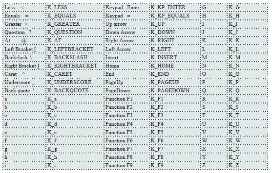
The parameters are not characters in the normal sense, but are numeric codes that can identify the character. These are based on the Pygame character constants, but extends them slightly. Table 9.1 gives a list of all of the constants provided by Glib. As an example, if a program must recognize when the up arrow key is pressed, the keyPressed () function that would do this is:
def keyPressed (k):
if k == K_UP:
print ("Up arrow key pressed.")
In an event-driven program it is unusual for key presses to be converted into strings, as they normally would be in a typical console-style program. That’s because it is expected that the interface to the event-driven program will be through mouse gestures and using single key commands from the keyboard, like “up
arrow” meaning “move forward.”
Example: Pressing a “+” Creates a Random Circle
This program will draw a circle at a random location when the “+” key is pressed. Old circles will remain. This illustrates the use of the keyboard in an obvious way. The initialization is to clear the screen and set the background color and fill color. The keyPressed() function generates random x,y coordinates and draws a circle there:
from Glib import *
from random import *
def keyPressed (k):
if k == K_PLUS:
ellipse (randrange(0,width), randrange(0,height), 30, 30)
startdraw(400, 400)
fill (200, 0, 0)
background (200)
enddraw()
The key value is passed as an integer, but the built-in function chr() will convert that to the proper character in many cases. What is possibly the shortest functional Glib program simply reads the keys and prints them on the console:
from Glib import *
def keyPressed(k):
print (chr(k))
startdraw()
enddraw()
The startdraw() function has default parameters, and creates a 50x50 pixel window if no size is specified. This program does not draw anything, so draw() is not needed.
Example: Reading a Character String
There are some reasons why an event-driven program might wish to read data from the user as a string. Perhaps a name is required, or a key value to access a database, or a password. Whatever the reason, it should be possible to read a string using keyPressed(). The way it would normally be done is to read one character at a time, normal for keyPressed(), and construct a string by concatenation. That’s how this program works:
from Glib import *
s = ""
t = ""
def keyPressed(k): # k is the value of the key that
# was pressed
global s, t
if k == K_RETURN: # Typing RETURN ends the string
# construction
t = s
s = ""
return
if k == K_BACKSPACE and len(s)>0: # Delete the
# previous character
s = s[0:len(s)-1] # Shorten the string by one
# character
else:
s = s + chr(k) # Append the new character to
# the string
def draw ():
global s, t
background (200)
text ("Enter a string: ", 10, 100)
text (s, 20, 130)
if (t != ""):
text ("Completed string is "+t, 20, 150)
startdraw(200, 200)
enddraw()
The global variable s holds the string being built, and the string t holds the final string. Characters are captured from the keyboard by keyPressed() and fall into one of three categories:
1. Most characters are added to the global string s through concatenation. The character passed to keyPressed() is an integer. The chr() function converts it to a character which is added to the end of s.
2. A BACKSPACE will delete the last character typed from the string. This is done using a substring from 0 to the second last character.
3. A RETURN will end the string. The current string in s will be assigned to t, and s will be reset to an empty string.
This kind of string data entry is especially useful when entering file names and numeric parameters. There are frequently special interface objects (widgets) that perform these tasks, such as text boxes. Glib could be used to implement such a widget (see: Exercise 6).
9.3 ANIMATION
Making graphical objects change position is simple, but making them seem to move is more difficult. Animation is something of an optical illusion; images are drawn in succession, and so quickly that the human eye can’t detect that they are distinct images. Small changes in position in a sequence of these images will be seen as motion rather than as a set of still pictures. A typical animation draws a new image (frame) between 24 and 30 times per second to make the illusion work.
There are two kinds of animation that can be done using Glib. The first involves objects that consist of primitives that are drawn by the library. A circle can represent a ball, for instance, or a set of rectangles and curves could be a car. The second kind of animation uses images, where each image is one frame in the sequence. These images are displayed entirely in rapid succession to create the animation. In the first case the animation is being created as the program
executes, whereas in the second the animation is complete before the program runs, and the program really just puts it on the screen.
9.3.1 Object Animation
Animating an object involves updating its position, speed, and orientation at small time intervals, so all of these aspects of the object must be kept in variables. If there are many objects being animated, then all of these variables must exist for each object, and are updated at the end of each time interval. If the animation is displaying 30 frames per second, then a new frame is drawn every 0.03 seconds. In Glib the function named framerate() can be called passing the number of times that draw() will be called each second, and then draw() can do the work needed to update the objects and draw the frame.
Example: A Ball in a Box
Imagine a ball bouncing in a square box. A box has three dimensions, of course, but for this example it will be restricted to two, so it will look like a circle within a square. The ball is moving, and when it strikes one of the sides of the square it will bounce, thus changing direction. There is one moving object: the ball. Graphically it is simply a circle, with position x,y and speed dx in the x direction and dy in the y direction. It will have size 30 pixels. The box will simply be the window the circle is drawn in.
During each frame the ball will move dx pixels in the x and dy pixels in the y direction, so within the draw() function the position is updated as:
x = x + dx
y = y + dy
This new position is where to draw the circle. However, if the ball is outside of the box after it is moved, then a bounce has to be performed. That is, if the new position of x is, for instance, less than 0, then it would have struck the left side of the square and then changed x direction (bounced). In this case, and also if x>width, the bounce is implemented by:
dx = -dx
Similarly, if the y coordinate of the ball becomes less than 0 or greater than the height, then it bounces vertically:
dy = -dy
This would all be true if the ball were very tiny, a single point, but it has a size of 30 pixels, and the coordinates of the circle are the coordinates of its center. This means that the method described above will bounce the circle only after the center coordinate passes the boundary, meaning that half of the circle is already on the other side. It’s easy to fix: the ball is 30 pixels in size, so it should bounce when it gets within 15 pixels of any boundary. For example, the x bounce should occur when x<=15 or x>=width-15. The entire solution is:
# Bouncing ball animation.
from Glib import *
def draw ():
global dx, dy, x, y
background (200) # Erase the prior frame
x = x + dx # Change ball position
y = y + dy
if x<=15 or x>=width-15: # Bounce in X direction?
dx = -dx
if y<=15 or y>=height-15: # Bounce in Y direction?
dy = -dy
ellipse (x, y, 30, 30) # Draw the ball
startdraw(200, 200)
x = 100 # Initial x position of the
# ball
y = 100 # Initial y position
dx = 3 # Speed in x
dy = 2 # Speed in y
fill (30, 200, 20) # Fill with green
enddraw()

Eight frames from this animation showing the ball bouncing in a corner of the box are shown in Figure 9.2. An entire second’s worth of frames (30) are given on the accompanying disc.
If there are many objects then all of the positions and speeds, and perhaps even shape, size, and color would have to be kept and updated during each frame. There are two usual ways to do this. In the first case the parameters are kept in arrays (lists). There would be an array of x coordinates, an array of y coordinates, of speeds, and so on. Each frame could involve an update to all elements of the arrays. Updating the position can be done like this:
for i in range(0,Nobjects):
x[i] = x[i] + dx[i]
y[i] = y[i] + dy[i]
The other usual method for handling multiple objects is to create an object class that contains all of the parameters needed to display the object. There is still an array, but it is an array of object instances, and if it is cleverly programmed the class can be updated by calling an update() method:
for i in range(0,Nobjects):
ball[i].update()
Example: Many Balls in a Box
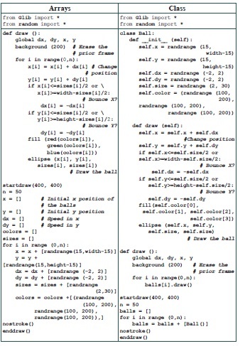
This example uses the same premise as the previous one, but will draw many balls in the window, all of them bouncing. Both methods for keeping track of objects, arrays, and classes will be illustrated. The many arrays solution has lists for x and y, for dx and dy, for color and for size. All parameters are initialized at random when the program begins.

The solution that uses classes defines a class ball within which the position, speed, color, and size are defined. The constructor initializes the values, and the update method changes the ball’s position and performs any needed bounces. The two solutions are:

These two solutions illustrate how classes work very neatly. The class contains individual properties of a ball and many are created; the arrays contain many instances of each property. So x[i] and ball[i].x represent the same thing. In this case the two programs are about the same size, but the class-based implementation encapsulates the details of the ball and what can be done with it. The class-based draw() function only says “draw each ball,” but in the array implementation the draw() function looks at all of the details of all balls to draw them. One of the implications is that it would be possible to divide the labor between two persons, one who wrote the class and another who wrote the rest of the code. For large programs this can matter quite a lot.
9.3.2 Frame Animation
The hard work in frame animation is done before the computer program is written. An animator has created drawings of an object in various stages of movement. All the program does is display frames one after the other, often looping them to create the desired effect. A common example of this is the animation of gait, walking or running. An artist draws multiple stages of a single step, being careful to ensure that timing is correct: how long does it take for a normal person to stake a pair of steps (left, right)? This time should agree with the frames the artist creates. If it takes one second to make the step, then it should be drawn as 30 frames.
Other kinds of animation are performed too. A fire can be animated as a very few frames, as can smoke and water. The program that draws the animation reads all of the image files into a collection. When the animation is played, the program displays one image after another within the draw function. This can be complicated by the fact that there may be multiple animations playing at the same time, possibly of different lengths and frame sizes.
Example: Read Frames and Play Them Back as an Animation
In this example there are 10 drawn animation frames of a cartoon character walking. These frames are intended to represent a single gait cycle, and so should be repeated. The program will do the following: when the up arrow key is pressed and held down, the character drawn in the window will “walk”; otherwise a still image will be displayed.
First the images should be read in and stored in an array (list) so that they can be played repeatedly. Then the keyPressed() function should be written so that when the up arrow key is pressed the frames will be drawn. A flag can be set True when the key is pressed, and False when the key is released so that draw() can tell when to draw frames and when not.
def keyPressed (k):
global keydown
keydown = True
def keyReleased(k):
global keydown
keydown = False
A list named frames is initialized with all of the images in the sequence. All that draw() does is play the next one, using a global variable f to identify the current frame.
def draw ():
global keydown, f
if keydown:
image (frames[f], 0, 0)
f = f + 1
if (f > 10):
f = 1
It cycles through the frames and repeats when all have been displayed.
The initialization can be a simple matter of reading ten images into variables and creating a list. This code does it in a loop, using a number in the name and incrementing it:
startdraw(320, 240)
keydown = False
frames = []
for i in range (1, 10):
s = "images/a00"+str(i) +".bmp"
x = loadImage (s)
frames = frames + [x,]
x = loadImage ("images/a010.bmp")
frames = frames + [x,]
x = loadImage ("images/a011.bmp")
frames = frames + [x,]
f = 1
image (frames[0], 0, 0)
enddraw()
The variable frames is a list holding all of the images, and frames[i] is the ith image in the sequence.
The building of the file name is interesting. It is common to use numbered names for animation frames; things like frame01, frame02, and so on. In this case the sequence is a***.bmp where the *** represents a three-digit number. If the variable i is an integer, then str(i) is a string containing that integer, but leading zeros are not present. Thus, for values of i between 0 and 9 (one digit), the string will be “a00”+str(i)+“.bmp”; for values of i between 10 and 99 (two digits), the string will be “a0”+str(i)++“.bmp”; finally, for numbers between 100 and 999, the string will be “a”+str(i)+“.bmp” (three digits). The leading zeros are manually inserted into the string.
The animation frames for the gait sequence are on the disk along with this code.
Example: Simulation of the Space Shuttle Control Console (A Class That Will Draw an Animation at a Specific Location)
Animations can sometimes be used to decorate a scene in interesting ways. A control panel showing video screens and data displays could use animations to fill the screens, giving the illusion of real things being monitored. A class that can play a frame-by-frame animation at any location on the screen could be instantiated many times, once for each display.
The class would have to read the frames it was to play and store them, play back the frames in a loop when requested, and place them within the window at any location. None of these tasks is especially hard. Code for reading frames from a file was written for the previous example, as was code for displaying the frames. Each class instance would need a frame count so that the loop could start over at the right place, and each class instance could have an animation with a different number of frames. Finally, placing at the right location is a matter of passing the correct parameters to the image() function. The class would be instantiated given the position as x and y coordinates of the upper left corner.
Sometimes, especially when multiple animations are playing, it will be necessary to slow down some animations so that they look right. The Glib code calls draw() a fixed number of times each second, but that may not always be the correct speed for an animation. A count can be introduced so that the frame advances to the next only when a count exceeds a fixed delay value. If the count is 2, for example, then 2 calls to draw() are required before a new frame is chosen, meaning that the frame rate has been decreased by 50%.
The specific example is supposed to implement a “simulation” of a space shuttle control console. This is a visual simulation, not one that allows interaction at any level, and the idea is to insert animations into a still photo of a real shuttle console and make it look more active. Figure 9.4a shows the static image that will be used. There are many video screens visible, and the program being developed will replace the still image on some of those screens with moving, animated images.
Three of the screens are selected for animation. The image was displayed using Paint and the coordinates of the upper left corner of each of these screens was determined, as were the sizes. Figure 9.4b shows the location of these regions on the image.
The code for the class starts like this:
class Anim:
def __init__ (self, x, y): # Constructor -------------
self.frames = [] # The actual images
self.xpos = x # Position of upper left
self.ypos = y
self.n = 0 # How many frames are there?
self.f = 0 # Which frame is currently
# being shown?
self.active = False # Is this animation being
# played?
self.delay = 1 # Used to slow the frame
# rate
self.count = 100000 # When count>delay a frame
# is drawn
def draw (self):
if self.active: # Draw the current frame at the
# correct location
image (self.frames[self.f], self.xpos, self.ypos)
self.count = self.count + 1 # Increment count.
if self.count >= self.delay: # Change the frame
# yet?
self.f = self.f + 1 # Yes. And also
# reset the count
self.count = 0
if (self.f >= self.n): # Loop the frames;
# start over at 0
self.f = 0
The part of the class that reads the frames as images is basically taken from the previous example:
def getframes (self, s1, s2):
self.frames = [] # The list variable
#'frames' contains all
# images
for i in range (0, 100): # Up to 100images can be
# read.
if i<10:
s = s1 + "0"+str(i) + s2
print ("Reading ", s)
elif i<100:
s = s1 + str(i) + s2
x = loadImage (s)
if x == None:
self.n = i
print ("Saw ", self.n, " frames.")
break
self.frames = self.frames + [x,]
There is a flag named active that determines whether the animations are currently running or not. The methods start() and stop() turn the animation on and off by toggling this variable.
def start(self):
self.active = True
def stop (self):
self.active = False
Finally, for this class, the delay can be set using a call to the setdelay() method, which simply changes the value of a class local variable delay.
def setdelay (self, d):
self.delay = d
The draw() method of the program simply draws the
animations by calling their respective draw() methods:
def draw ():
a.draw()
b.draw()
c.draw()
The main program opens the window and loads and draws the background image:
startdraw(800, 531) # The size of the background image
background = loadImage ("images/800px-STSCPanel.jpg")
image (background, 0, 0)
The first animation, at x=239 and y=284, will show some television static, seven frames of which were created for this purpose using another program.
A class instance is created to draw at (239,284) and getFrames() is called to load the images (the file names are “g100.gif ” through “g106.gif ”):
a = Anim(239, 284)
a.getframes ("images/g1", ".gif")
The second animation is at x=319 and y=258 and will display some exterior shots of the space shuttle. The process is the same as before, but the file names are “g200.jpg” through “g204.jpg.” In addition, a delay of 100 is set, because these images are to be displayed for multiple seconds each to simulate a display scanning a set of cameras:
b = Anim (319, 258)
b.getframes ("images/g2", ".jpg")
b.setdelay(100)
Finally the third animation, at x=319 and y=322, consists of a computer display showing Python code (this class, in fact). It was created by another program and consists of nine frames named “g300.gif” through “g308.gif.” This animation is delayed a little as well so that it appears as if the text is scrolling properly:
c = Anim (319, 322)
c.getframes ("images/g3", ".gif")
c.setdelay(10)
The last step in the program is to start all of the animations playing:
a.start()
b.start()
c.start()
enddraw()
The example is complete on the disk, and needs to be executed with the images directory, which contains the animation frames.
https://commons.wikimedia.org/wiki/File:STSCPanel.jpg
9.4 RGBA COLORS – TRANSPARENCY
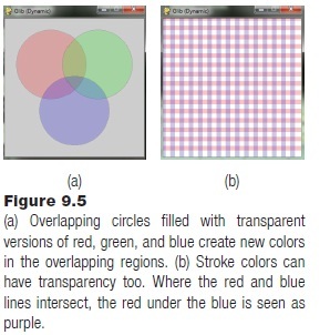
In Chapter 7, it was seen how it was possible to use transparency in an image to allow the visualization to ‘see through’ to an image in the background. As it happens, any pixel can be assigned a degree of transparency that permits the same visual character. A color can be assigned a value that dictates how opaque or transparent it is, allowing colors behind it to influence how that pixel is seen. One can think of this as a fourth color value, in addition to red, green, and blue. It is referred to as alpha, and a color with four color parameters is said to be in the RGBA color space, for Red, Green, Blue, and Alpha.
If the value of Alpha is 255, then the color is opaque; as it decreases in value the transparency increases until at Alpha=0 pixel or object cannot be seen. A program that draws three overlapping circles using colors with an Alpha value of 60 shows the visual effect of using transparency (Figure 9.5a). Transparency is specified in this case by providing the Alpha value as a fourth parameter to fill():
from Glib import *
startdraw(300, 300)
fill (255, 0, 0, 60)
ellipse (100, 100, 150, 150)
fill (0, 255, 0, 60)
ellipse (200, 100, 150, 150)
fill (0, 0, 255, 60)
ellipse (150, 200, 150, 150)
enddraw()
Transparency can be added to stroke colors also, and in the same way (Figure 9.5b). For example:
stroke (255, 0, 0, 65)
9.5 SOUND
Sound is an essential component of digital media. Proof? Almost nobody watches silent films anymore, and nobody makes them. Video games are rarely played with the sound turned off. There are a few important reasons for this.
1. Much human communication is through sound. Speech is the best example, but non-speech sounds, clapping, stamping of feet, and so on, are ways that people make their feelings and intentions known.
2. Sounds are associated with events. When an object falls to the floor a sound occurs with the impact. A button is pressed and a doorbell rings. These sounds are important indicators.
3. Sounds cause emotional reactions in people. Music can do this; it can convey a mood better than almost anything else. But sound can also indicate things unseen. A growling in the dark; a screech in the sky; the sound of an approaching vehicle around a curve in the road.
In Glib a sound is much like an image in terms of how it is used. A sound file is loaded and assigned to a variable, then that variable can be used to play, stop, rewind, and perform all audio operations on that sound. Each sound must be loaded into a distinct variable and has its own controls. The Glib interface to sounds files should therefore look familiar.
One problem is that the sound system does not have a large variety of sound files that it can handle: “.wav” and “.ogg” are about it. This leaves the more popular format, “mp3,” out of contention for Python media software, at least for now.
The first step in playing a sound is to load the file. The function loadSound() is used for this, passing the name of the sound file:
s = loadSound ("song.wav")
Playing the sound is done using the playSound() function of Glib:
playSound (s)
Stopping a sound from playing is a matter of calling stopSound(). Setting the volume means calling volumeSound() passing a parameter between 0.0 and 1.0, where 0.0 is no sound and 1.0 is maximum volume. That’s pretty much it for the basics.
Example: Play a Sound
The act of reading and playing a sound file will illustrate the essential operations for using sound. The file input is done as an initialization. Starting to play the file could be done that way too. Calling playSound() repeatedly from draw() will cause the file to start playing over and over again. A solution is to start some sounds in the main program; another is to set a flag when a sound starts playing and check the flag. The best way would be to record the time when the sound started playing and see if the current time exceeds the length of the sound.
If playSound() is called with a second parameter, an integer, then the sound will be replayed or repeated that many times. The call playsound(s, 3) plays the sound s three times. If the requested file does not exist, then loadSound() returns None.
Example: Control Volume Using the Keyboard. Pause and Unpause
This example adds volume control. The function volumeSound() accepts a single parameter, and it is a number between 0.0 (lowest volume) and 1.0 (highest volume). Adding a volume control is as simple as coding a keyPressed() function that changes the volume level by an increment each time a key is pressed. Use “+” for a volume increase and “-” for a decrease. The new program is:
from Glib import *
def keyPressed(k):
global volume, s
if k == K_PLUS:
volume = volume+.1
elif k == K_MINUS:
volume = volume-.1
if volume<0: volume = 0
if volume>1: volume = 1
volumeSound(s, volume)
startdraw()
s = loadSound ("sun.wav")
volume = 1.0
volumeSound (s, volume)
if s == None:
print ("No such sound file.")
else:
playSound(s)
enddraw()
Example: Play a Sound Effect at the Right Moment: Bounces
A sound effect represents some event, and needs to be played at the moment the event happens. Synchronizing the two things is as simple as playing a sound when the event is detected. This example program will play a sound representing a ball hitting something when a simulated ball hits the side of the window and bounces. The bouncing ball animation program will provide the impact event: when the ball hits the side of the window, the sound of an impact will be played.
The sound effect is a file, and was recorded using an inexpensive microphone, a computer with a sound card, and the Audacity software, which is free and downloadable (see the end-of-chapter resources). The sound of a glass hitting a desk was recorded, edited, and saved as a “.wav” file named “bounce.wav.” The program was modified to read that file, and then play it back whenever a collision with the window was detected. The program has three new lines of code:
# Bouncing ball animation.
from Glib import *
def draw ():
global dx, dy, x, y
background (200) # Erase the prior frame
x = x + dx # Change ball position
y = y + dy
if x<=15 or x>=width-15: # Bounce in X direction?
playSound (s)
dx = -dx
if y<=15 or y>=height-15: # Bounce in Y direction?
dy = -dy
playSound(s)
ellipse (x, y, 30, 30) # Draw the ball
startdraw(200, 200)
x = 100 # Initial x position of the
# ball
y = 100 # Initial y position
dx = 3 # Speed in x
dy = 2 # Speed in y
s = loadSound ("bounce.wav")
fill (30, 200, 20) # Fill with green
enddraw()
In many situations there can be a small delay between the event and the sound being played. A sound can rarely be played instantaneously.
9.6 VIDEO
The video facilities provided by Glib are limited, but the library increases the functionality of the underlying Pygame module. It is important to understand that video plays at a particular rate and, unlike audio, must acquire a portion of the display window within which to be drawn. This means that playing a video in the normal way takes control away from the programmer and allows the video software autonomy. This can cause some trouble, as programmers often want to draw into the display window as well.
Using the basic functionality it is possible to play an MPEG-formatted video with sound anywhere in the window, and the window can be sized to suit the purpose. Only a single video can be played in this way at one time, though. A video has characteristics of both sounds and images: the video resides in a file; it is placed in a specific location in the window, and has a two-dimensional size (a width and height), but the image displayed changes as a function of time. Also, a video can have sound as one of its properties. However, because multiple videos may have multiple sound channels, only one of them is given the sound output channel, meaning that only one can play sound.
A video is read into a variable in the same way as an image or sound: a function loadVideo() returns a variable that references the data on an MPEG file which is specified by file name as the parameter. A video is played by calling the function playVideo() and passing the value returned by loadVideo(). The smallest program that plays a video file would be something like this:
from Glib import *
startdraw(400, 400)
s = loadVideo ("ellipsis.mpg")
if s != None:
playVideo(s)
enddraw()
The file being opened and played is one provided on the accompanying
disc, “ellipsis.mpg,” and it has no sound. The variable s represents the video in the program, and is returned by loadVideo(). It is, in fact, a reference to a Glib class named Gvideo. If it has the value None, then no video file was loaded for some reason: perhaps the file does not exist or is in a format that can’t be processed. Glib only recognizes MPEG video files, and even then only MPEG I. The playVideo() function places the image in the upper left corner of the window and begins playing it, sound included.
There are a small collection of useful functions in Glib for dealing with videos. They are:
pauseVideo(m): Parameter m is a video. Pauses the video if it is playing or resumes it if it is paused
stopVideo (m): Parameter m is a video. Stops playing the video m
rewindVideo (m): Parameter m is a video. Returns the video to the beginning
isVideoPlaying (m): Parameter m is a video. Returns True if the video is playing
setVideoVolume(m, v): Parameter m is a video. Adjusts the audio volume on the video m to be the value v, where v=0 is the minimum and v=1.0 is the maximum
lengthVideo (m): Parameter m is a video. Returns the length of the video in seconds
whereVideo(m): Parameter m is a video. Returns the current location in the video, in seconds from the start
getVideoFrame(m): Parameter m is a video. Returns the current video frame playing
setVideoFrame(m, f): Parameter m is a video. Changes the playback so the next frame in the video to play is frame f
getVideoPixel(m, x, y): Parameter m is a video. Returns the value of the pixel at location (x,y) in the frame currently being displayed
sizeVideo (m): Parameter m is a video. Returns the dimensions of a video frame. The video must be loaded
videoSize (s): Parameter s is a string. Returns the dimensions a frame in the video file s, where s is a string. Use this for finding the size before loading the file
locVideo (m, x, y, w, h): Position the video m at position (x,y) in the window, and make it wxh pixels in size. Does not start it playing
Example: Carclub – Display the Video carclub2.mpg (Annotated)
When the p key is pressed the video will pause, and when pressed again it will resume. Display the video at location 100, 100 in the window and make it 200x200 pixels. Display the number of the current frame and the current time of the frame being played.
This program uses eight of the fifteen video functions. First the file is loaded and the location and size are set using locVideo(). Then the main program starts the video playing.
The draw() function is responsible for updating the numeric values displayed. It resets the background and then checks to see if the video is playing; it displays “Playing” if so, or “Not playing” otherwise. The current position, current time, and total time are extracted and displayed using calls to text().
Finally the pause feature is implemented. In the function keyPressed() the function checks that the key pressed was “p,” and if so it calls pauseVideo(). This function keeps track of whether or not the function is playing and knows whether to start or stop the video. Here is the program:
from Glib import *
def draw ():
global vid
background (0, 200, 190) # Clear the background,
# set to aqua.
if isVideoPlaying(vid): # Playing? Print an
# indicator
text ("playing", 10, 40)
else:
text ("Not playing", 10, 40)
whr = whereVideo(vid) # Current time of play
text ("Frame "+str(getVideoFrame(vid)), 10, 60)
# Current frame
text ("Length "+ str(whr)+" of "+str(lengthVideo(vid)),
40, 370)
def keyPressed(k):
global vid
if k == K_p: # Key pressed was a 'p'
pauseVideo(vid) # Pause
startdraw(500, 500)
vid = loadVideo("carclub2.mpg") # Load the car club video
locVideo(vid, 100, 100, 200, 200) # Position it at
# (100, 100)
playVideo(vid) # Play it.
enddraw()
A screen shot of this program in action is shown in Figure 9.5. Note that the current time is displayed to 16 or so digits. This can be changed to display something more reasonable (see: Exercise 8).
There are four different ways to “play” a video using Glib, and each has a distinct set of pros and cons and a process for how to manage the video. After loading the video into variable m:
1. Using the Glib functions – loadVideo(), locVideo(), play() and so on isolate the programmer from the actual video class Gvideo. These are typically used when there are one or two videos and there is no complicated processing going on. Only one video with sound can be played; the others will play muted.
2. AutoPlay(m) – The video m will play automatically in the current display window. The user has some control: the video can be paused and can be located at a specific location and size. It will play at the internally designated rate (frames per second) with sound. Only one video with sound can be played in this way; the others will not have the sound played.
3. PlayVideo(m) – The video will play at its internal frame rate, but a frame will not be displayed until the drawVid() function is called. If drawVid() is called inside of the user’s draw() function then the frames will be displayed at the Glib-specified frame rate, but some video frames might be missed.
4. DrawFrame(m, f) – The frame numbered f of the video m will be drawn. Sound will not play. This permits the best control of the video, because each frame can be played at any speed without missing any; or, every second or third frame can be played; or random frames can be played. The video can even be played backwards – simply start f at the largest frame value and decrease by 1 each time.
Three of these different styles are illustrated in the table below:


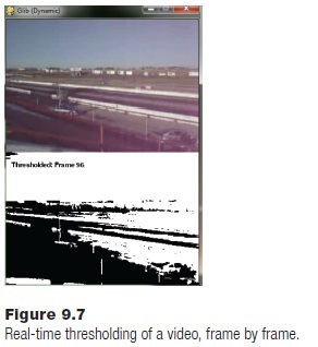
Exercise: Threshold a Video (Processing Pixels)
In Chapter 7, a program was written that thresholded an image. It converted each pixel to a grey value and if that value was smaller than a specified threshold it would be set to black; otherwise it would be set to white. Each frame of a video is an image, and it should be possible to threshold each frame and then display it. Glib provides the getVideoPixel() function that returns the value of a specified pixel in the current frame of a video.
This example will use draw_frame() to display the video, and draw_frame() will be called from the user’s draw() function. After the frame is displayed each pixel in the frame is examined (getVideoPixel ()), converted to a grey value (grey(p)), and tested against a threshold; if smaller than the threshold, it will be drawn as black by calling fill (0) and drawing the pixel with point (). Otherwise, the pixel will be drawn as white. The original image is displayed at the top of the window, the thresholded one below. Thus the window has to be created initially with double the height of the image to make room for two copies.
from Glib import *
def draw ():
global frame, v, wid, ht, x
background (200)
draw_frame(v, frame)
for j in range(0,ht):
p = getVideoPixel (v, i, j)
g = grey(p)
if g<t:
fill (0)
else:
fill (255)
point (i, j+ht)
frame = frame + 1
fill (0)
text ("Original: Frame"+str(frame), 10, 30)
text ("Thresholded: Frame "+str(frame), 10, ht+30)
s = videoSize("carclub2.mpg")
startdraw(s[0],s[1]*2)
v = loadVideo ("carclub2.mpg")
frame = 1
wid = s[0]
ht = s[1]
t = 100
locVideo(v, 0, 0, wid, ht)
enddraw()
9.7 SUMMARY
A facility has already been described for displaying images and graphics: Glib, and here more media capability is added to Glib, thus building on what has already been discussed, so that sound and video can be displayed. The new
library is dynamic Glib and offers the same functionality as previously plus sound, animation, and video.
Using mouse position and button presses is a basic form of communication with a computer. The Glib module keeps track of the mouse using Pygame and continually updates the position as two variables: mouseX and mouseY hold the most recent x and y coordinates. If the user writes a function named mousePressed(), then it will be executed when a mouse button is pressed. Similarly, when a mouse button is released it tries to call mousereleased(). A software graphical button is a rectangle or other area which, if the mouse button is clicked while the mouse cursor is within that area, will perform a task; in other words, the click while the cursor is in that area calls a function.
The keyboard is similarly dealt with by having a user-coded function keyPressed() and another named keyReleased(). They are passed the value of the key that was pressed as the parameter.
Animation is performed by rapidly displaying drawn images, or frames, one after the other, or by creating and drawing graphical objects and then changing their positions. A function named draw() can be written by the programmer to draw the frames many times each second.
Sounds are displayed by reading them from a file and calling a play() function when the sound is needed. Sounds can be music, voice, ambiance, or sound effects.
Video is the most resource-consuming of the media types. Glib allows videos to be recalled and placed in the window, and to be played automatically or frame by frame.
Exercises
1. Write a program that figures out how fast the mouse is moving (pixels per second assuming 30 frames per second) and displays that value.
2. Consider the example that prints a circle at a random position when a “+” key is pressed. Modify it so that when the “-” key is pressed, the previous circle is deleted (no longer appears on the screen).
3. Write a program that reads lines from a file as pairs of x,y coordinates on a single line and draw them all. Each line would have four integers:
100 100 200 200
which are the (x,y) coordinates of the start and endpoints of the line. In the example above, the line would be drawn between (100, 100) and (200, 200).
4. Implement a circular button. It is represented on the screen as a circle at (100, 100) of size 30 pixels. Normally it is red, but it turns green when activated. When a mouse button is pressed while the button is activated, a rectangle is drawn somewhere (random) in the window.
5. Implement a button that normally has the text “Yes” drawn within it, but that changes that text to “No” when the button is activated. Pressing it does nothing.
6. Use Glib to implement a text box that permits a file name or other text to be entered when the mouse cursor is within that region defined by the box. Use this to create a program that allows the user to enter a file name of an image and have the program display this image in the window.
7. Modify the program from Exercise 5 above so that a sound is made when the button is pressed. A clicking sound would be most appropriate, but whatever it is it must be of short duration.
8. Floating point values, such as the current time of the video in seconds, are often converted into strings and require ten or more digits to be displayed. Write a function that changes a floating point number so that it will display in five digits, and modify the video display program named carclub so that all floats are displayed with only two digits to the right of the decimal.
9. Modify the simulation of the space shuttle console so that videos are played in the simulated screens instead of frame-by-frame animations.
Notes and Other Resources
Thanks to the estate of composer and musician and friend Michael Becker for the use of the song ‘Holding On,’ and for the use of the .wav file.
Download for the Pygame module. http://www.pygame.org/download.shtml
An excellent sound editor for .wav and .mp3 files. http://www.goldwave.ca/
Another excellent sound file editor. http://sourceforge.net/projects/audacity/
Complete Pygame documentation. https://media.readthedocs.org/pdf/pygame/latest/pygame.pdf
Convert video files into MPEG-I format. http://video.online-convert.com/convert-to-mpeg-1
A good tutorial on video formats. http://www.videomaker.com/article/c10/15362-video-formats-explained
Free software that converts between video formats. http://www.any-video-converter.com/products/for_video_free/
1. Al Sweigart. (2012). Making Games with Python & Pygame, CreateSpace Independent Publishing Platform, ISBN-13: 978-1469901732.
2. Sean Riley. (2003). Game Programming with Python, Charles River Media.
3. Vic Costello. (2016). Multimedia Foundations, 2nd edition, Focal Press, ISBN-13: 978-0415740036.
4. Richard Boulanger and Victor Lazzarini (Eds.). (2010). The Audio Programming Book, The MIT Press, Har/DVD edition, ISBN-13: 978-0262014465.
5. Sendpoints. (2015). GUI: Graphical User Interface Design, ISBN-13: 978-9881383495.
6. Mahesh Venkitachalam. (2015). Python Playground: Geeky Projects for the Curious Programmer, No Starch Press, ISBN-13: 978-1593276041.

