
PROGRAMMING FOR THE SCIENCES
11.1 Finding Roots of Equations
11.2 Differentiation
11.3 Integration
11.4 Optimization: Finding Maxima and Minima
11.5 Longest Common Subsequence (Edit Distance)
11.6 Summary

In this chapter
It is true that the earliest calculating devices were created to help with commercial concerns, like payments, credit, and inventory. The abacus is an excellent example—it does basic arithmetic and was likely an early “cash register.” Much older devices do exist, such as the Lebombo bone that helped ancient African bushmen do simple calculations and keep track of time. The electronic computer, on the other hand, was designed to carry out scientific calculations, in particular those related to decrypting military messages and building the atom bomb. Computers are, of course, used for those things still, but there is now a vast array of computations in the scientific domain that could not be carried out without the help of a computer.
Scientists from different disciplines would disagree about what the most important algorithms and techniques for science were. That’s because of the widely disparate things that physicists and biologists, as two examples, study. There are a few recurring problems that pop up in almost all science domains, and some important techniques that generalize to many science and some non-science areas.
11.1 FINDING ROOTS OF EQUATIONS
The root of an equation is the x coordinate corresponding to its zero value. This may not be the smallest or the largest value, but the place where a function equals zero is often important. For example, if a function for the error in a calculation can be found, then finding the place where the error is zero would be important. In one dimension the problem being solved is:
x: f (x) = 0 (11.1)
Or in other words, find the value of x that results in f(x) being equal to zero. The function could be quite complicated, but for the technique to work it should have a derivative.
The basis of many root finding procedures is Newton’s method. The procedure begins with a guess at the right answer. The guess in many cases does not have to be very accurate, but is simply a starting point. If a range of values is given within which to find the solution, the center of that range may be a good starting guess. So, here is a problem to start with:
f (x) = (x-1)3 between x = -2 and x = 12 (11.2)
The center of the range is x = 5.
The initial guess is called x0, and here x0 = 5. The function value there, f(x0), is 64. The algorithm now says that the next guess for x, x1, will be:
x0 – f (x0)/f’(x0) (11.3)
where f’(x0) is the derivative of f at the point x= x0. This is a wrinkle—the derivative of f has to be calculated. It’s easy to do for many functions, hard for others. A numerical method will be examined a little later in this chapter, so in the meantime it is possible to simply code a function that gives the derivative, having done the calculus on paper and then written the function based on that. The derivative of (x-1)3 is 3x2 - 6x+3.
def objective (x):
return (x-1)*(x-1)*(x-1)
def deriv (x):
return 3*x*x - 6*x+3
# Range is -2 to +12
x = 5.
fx = 1000.
delta = 0.000001
print ("Step 0: x=", x, " obj = ", objective(x))
i = 1
while abs(fx) > delta:
f = objective(x)
ff = f/deriv(x)
x = x - ff
fx = objective(x)
print ("Step ",i,": x=", x, " obj = ", fx)
i = i + 1
Step 0: x= 5.0 obj = 64.0
Step 1 : x= 3.666666666666667 obj = 18.96296296296297
Step 2 : x= 2.7777777777777777 obj = 5.618655692729766
Step 3 : x= 2.185185185185185 obj = 1.6647868719199308
. . .
Step 14 : x= 1.0137019495631274 obj = 2.5724508967303e-06
Step 15 : x= 1.0091346330420865 obj = 7.622076731056633e-07
The correct answer in this case is x=1.0, so the method gets to within 0.009 of the correct root in 15 steps. Depending on the application, this could be fine. What if the initial guess was terrible? If the process starts at x = 500 then it takes 27 steps, but gets just a little closer to the right answer (x=1.0087). Starting at -500 also takes 27 steps.
It’s possible that there is no root. What happens in that case? The program keeps looking. It overshoots, and then goes back, and forth, and back again. To present this from happening it is common to place a limit of the number of times the program will try. When this limit is exceeded an error occurs indicating that there is no solution.
This first example has illustrated some common concepts that are used in numerical analysis, which is the mathematical discipline encompassing the computation of mathematical functions and operations. The common concepts include:
The initial guess: It is relatively common to have a numerical algorithm begin at a guessed value.
The delta: It is also common to have an algorithm step when the change in the result or some mathematical feature becomes smaller than a specified threshold, called delta.
Iteration: Numerical methods frequently repeat a calculation expecting it to converge on the correct result, using the previously calculated value as the new starting point.
Maximum iterations: A user of a numerical method can assume that the method will not converge (get close enough to the right answer) if a specified number of attempts have been made.
11.2 DIFFERENTIATION
Determining the derivative of a function is something that is often thought of as a symbolic operation, and the result is valid for any value of the function. This may not always be true, and it may not be easy to do in the general case. Think about what the previous algorithm does—it needs the derivative of a function at one specific point. Can that be determined if the algebraic form of the function is not known? Yes, it can, to within some degree of accuracy.
The derivative of a function at a point x is the slope of the curve defined by that function at that point. The definition of the derivative of f at the point x is:
f ’(x) = (f (x + h) – f (x - h))/(2h) (11.4)
as h gets smaller and smaller, what is called a limit in calculus. This formula is essentially the mathematical definition of a derivative. On a computer h can be made quite small, but can never be zero. If the expression above is used as an estimate of the derivative, it will work in many cases. It is based on sampling two points of the function each time. An improvement can be made by using more points; for example:

uses four points and often produces better results.
Coding this uses a function passed as a parameter. It makes sense that the function to be differentiated would be a parameter to the function that differentiates it; other parameters will be x, the point at which it will be evaluated, delta, the accuracy desired, and niter, the maximum number of iterations. The calculation should take place in a try-except block so that numerical errors will be caught. The two-point and the four-point versions of the function that performs numerical differentiation are:
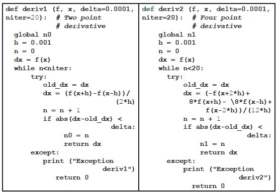
Testing these functions is an excellent demonstration. First a function to be differentiated is written. The previous example on finding roots has a simple one (renamed as f1):
def f1 (x):
return (x-1)*(x-1)*(x-1)
That example also has a function that represents the derivative of f1 at the point x (renamed df1):
def df1 (x):
return 3*x*x - 6*x+3
The function df1() should return the exact derivative of f1(), and can be used to check the value returned by deriv1() or deriv2(). Create a loop that runs over a range of x values and compare the value returned from df1() to that returned by deriv1() and/or deriv2():
for i in range (1,20):
x = i*1.0
f = f1(x)
df = df1(x)
mydf = deriv1 (f1, x)
mydf2 = deriv2(f1, x)
print (f, df, mydf, n0, " ", mydf2, n1)
The result looks something like this:

Both functions give excellent results in a very few iterations in this case. Of course, some functions present more difficulties than do simple polynomials. [2]
11.3 INTEGRATION
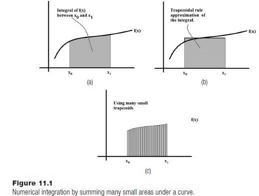
An integral is most often thought of as the area under a curve, where the curve is a function (Figure 11.1a). Numerical integration amounts calculating that area using an algorithm. The area of a rectangle is easy to calculate, so if the region under a curve could be reasonably approximated by a bunch of rectangles, then the problem would be solved. This is the idea behind the trapezoidal rule. The integral from x0 to x1 of a function f(x) can be approximated by the width (x1 - x0) multiplied by the height (the average value of the function in that range), which is just a rectangle that approximates the area under the curve (Figure 11.1b). In mathematical notation:

This would generally be a pretty poor approximation of a curve, and would yield correspondingly bad approximations of the integral. However, the smaller the width x1 - x0 the more accurate the approximation can be, and so using a great many small trapezoids would be much better than using only one (Figure 11.1c). How many? That is not known at the outset, but could be increased from an initial guess until a desired accuracy was achieved.
A function that performs integration using this method would accept a function, the starting x0 and the ending x1 for the integral. The function would break the interval between x0 and x1 into n parts, when n is an initial guess. The function is evaluated for all n parts, the area of each trapezoid is computed, and they are summed to get the final result. Now increase n and do it again. If the two values are close enough (delta) then the process is complete.
This will be done in two steps. First a function trap0() that computes and returns the sum of N trapezoids. The obvious but slow way to do this is:
f trap0 (f, x0, x1, n): # Slow method
dx = (x1-x0)/n # Divide range into N parts
xa = x0 # Start at x0
xb = x0+dx # Current trapezoid is xa to xb
sum = 0 # Sum of areas starts at 0.0
for i in range(0, n): # Add up N trapezoids
f0 = f(xa) # Compute function at xa and xb
f1 = f(xb)
sum = sum + dx*(f1+f0)/2 # Area of the trapezoid
xa = xa + dx # Next xa and xb are dx from
xb = xb + dx # the current ones
return sum # The sum is the integral.
The integration function trapezoid() will call this function with increasing values of n until two consecutive results show a small enough difference (i.e., smaller than a provided delta value):
def trapezoid (f, x0, x1, delta=0.0001, niter=1024):
n = 4
resold = trap0(f, x0, x1, 2)
resnew = trap0(f, x0, x1, 4)
while abs(resnew-resold) > delta:
if n>niter: break
resold = resnew
n = n * 2
resnew = trap0 (f, x0, x1, n)
return resnew
The function trap0() can be sped up significantly by not re-computing the function twice each time through the loop, but remembering the previous value instead (Exercise 2). A more popular algorithm for integration is Simpson’s Rule, which tries to minimize the error even more by using a quadratic approximation to the curve at the top of the trapezoid, instead of a straight line.
11.4 OPTIMIZATION: FINDING MAXIMA AND MINIMA
Finding extreme values, either the maximum or minimum, is a very common problem in computing, not just in science but in many disciplines. It is sometimes referred to as optimization. Naturally finding a best (in some sense) value would be appealing. What is the least amount of fuel needed to travel from Chicago to Atlanta? What route between those two cities requires the least amount of driving time? What route is shortest in terms of distance? There are many reasons to want an optimum and many ways to define what an optimum is.
In the following discussion the function to be optimized will be provided, so there will no guesswork on that subject. The question concerns how to find location (parameters) where the minimum or maximum occurs.
11.4.1 Newton Again
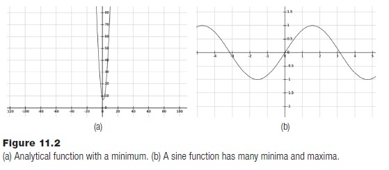
Figure 11.2 shows an example of a function to be optimized. There is a minimum of 7 at the point x= 1. How can this be found? If the nature of the function is known, for instance that it is a quadratic polynomial, then the optimum can be found immediately. It will be at the point where the derivative is zero. The problem of optimization is that one does not know much, if anything, about the function. It can only be evaluated, and perhaps the derivatives can be found numerically. Given that, how can the min or max be found?
If the derivative can be found, then it may be possible to search for an optimum point. At a value x, if the derivative is negative, then the slope of the curve is negative at that point; if the derivative is positive then the slope is positive. If an x value can be found where the slope is negative (call this point x0) and another where it is positive (call this x1), then the optimum (slope = 0) must be between these two points. Finding that point can be done as follows:
1. Select the point between these two (x = (x0+ x1)/2).
2. If the derivative is negative at this point, let x0 = x. If positive let x1 = x.
3. Repeat from step 1 until the derivative is close enough to 0.
This process is pretty much random. Finding the two starting points is a matter of guessing until they are found. The search range gets smaller by a factor of 2 each iteration. The fact that the function can be evaluated at any point means that it is possible to make better guesses. In particular, it’s possible to assume that the function is approximately quadratic at each step. Quadratics have an optimum at a predictable place. The method called Newton’s Method fits a quadratic at each point and moves towards its optimal point.
The method is iterative, and without doing the math the iteration is:

A function to calculate the first and second derivative is needed. The formula for the second derivative is based on the definition of differentiation, as was the formula for the first. It is:

The program should therefore be straightforward. Repeat the calculation of xn-1 - f’(x)/f’’(x) until it converges to the answer. This will be the location of the optimum. An example function would be:
def newtonopt (f, x0, x1, delta=0.0001, niter=20):
x = (x0+x1)/2
fa = 1000.0
fb = f(x)
i = 0
print ("Iteration 0: x=", x, " f=", fb)
while (abs(fa-fb) > delta):
fa = fb
x = x - deriv(f, x)/derivsecond(f, x)
fb = f(x)
i = i + 1
print ("Iteration ", i, ": x=", x, " f=", fb)
if i>niter:
return 0
This finds a local optimum between the values of x0 and x1. A local optimum may not be the largest or smallest function value that the function can produce, but may be the optimum in a local range of values.
Figure 11.2a shows a typical quadratic function. It is f(x) = x2-2x+8, and has an optimum at x = 1. Because it is quadratic the Newton optimization function above finds the result in a single step. Figure 11.2b is a sine function, and can be seen to have many minima and maxima. Any one of them might be found by the Newton method, which is why a range of values is provided to the function.
The newtonopt() function successfully finds the optimum in Figure 11.2a at x=1, and finds one in Figure 11.2b at x = 90 degrees (π/2 radians). If there is no optimum the iteration limit will be reached. If either derivative does not exist, then an exception will occur.
11.4.2 Fitting Data to Curves – Regression
Scientists collect data on nearly everything. Data are really numerical values that represent some process, whether it be physical, chemical, biological, or sociological. The numbers are measurements, and scientists model processes using these measurements in order to further understand them. One of the first things that is usually done is to try to find a pattern in the data that may give some insight into the underlying process, or at least allow predictions for situations not measured. One of the common methods in data analysis is to fit a curve to the data; that is, to determine whether a strong mathematical relationship exists between the measurements.
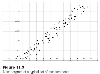
As an example, a set of measurements of tree heights will be used. The height of a set of a specific variety of trees is made over a period of ten years and the data resides in a file named “treedata.txt.” The question: is there a linear relationship (i.e., does a tree grow generally the same amount each year)? Specifically, what is that relationship (i.e., how much can we expect a tree to grow)? Figure z shows a visualization of these data in the form of a scattergram or scatter plot, in which the data are displayed as points in their (x,y) position on a grid.
The “curve” to be fit in this case will be a line. What is the equation of the line that best represents the data in the figure? If that were known then it would be possible to predict the height of a tree with some degree of confidence, or to estimate a tree’s age from its height.
One form of the equation of a line is the point-slope form:
y = mx+b
where m is the slope (angle) of the line and b is the intercept, the place where the line crosses the Y axis. The goal of the regression process, in which the best line is found, is to identify the values of m and b. A simple observation is needed first: the equation of a line can be written as:
mx + b - y = 0
If a point actually sits on this line, then plugging its x and y values into the equation will result in a 0 value. If a point is not on the line, then mx+b-y will result in a number that amounts to an error; its magnitude indicates how far away the point is from the line. Fitting a line to the data can be expressed as an optimization problem: find a line that minimizes the total error over all sample data points. If (xi,yi) is data point i then the goal is to minimize:

by finding the best values of m and b. The expression is squared so that it will always be positive, which simplifies the math. It may be possible to do this optimization using a general optimization process such as Newton’s, but fortunately for a straight line the math has been done in advance. Other situations are more complicated, depending on the function being fit and the number of dimensions.
A simple linear regression is done by looking at the data and calculating the following:
Each of these can be calculated using a separate function. Then the slope of the best line through the data would be:

And the intercept is:
b = meany – m*meanx (11.11)
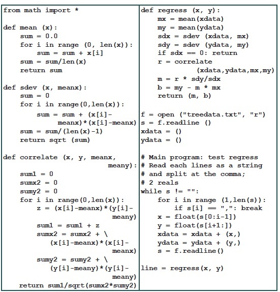
The function regress() that does the regression accepts a tuple of X values and a corresponding tuple of Y values, and returns a tuple (m, b) containing the parameters of the line that fits the data. It depends on other functions to calculate the mean, standard deviation, and correlation; these functions could generally be more useful in other applications. The entire collection of code is:
11.4.3 Evolutionary Methods
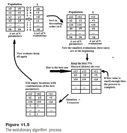
A genetic algorithm (GA) or an evolutionary algorithm (EA) is an optimization technique that uses natural selection as a metaphor to optimize a function or process. The idea is to create a collection of many possible solutions (a population), which are really just sets of parameters to the objective function. These are evaluated (by calling the function) and the best of them are kept in the population; the remainder are discarded. The population is refilled by combining the remaining parameter sets with each other in various ways in a process that mimics reproduction, and then this new population is evaluated and the process repeats.
The idea is that the population contains the best solutions that have been seen so far, and that by recombining them a new, better set of solutions can be created, just as nature selects plants and animals to suit their environment. This method does not require the calculation of a derivative, so it can be used to optimize “functions” that can’t be handled in other ways. It can also deal with large dimensions; that is, functions that take a large number of parameters.
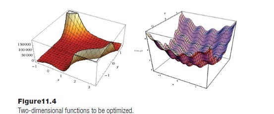
This idea may be new, and so developing it with an example may be the best way to illustrate it. Consider the problem of finding the minimum of a function of two variables. This is really an attempt to find values for x and y that result in the smallest function result. Evolutionary algorithms are often tested on quite nasty functions, having lots of local minima or large flat regions. Two such functions will be used here: the Goldstein-Price function:
(1+(x+y+1)2 (19 - 14x+3x2 - 14y + 6xy+3y2) (30+(2x+3y)2 (18 - 32x+12x2+48y - 36xy+27y2)) (11.12)
and Bohachevsky’s function:
x2 + y2 – 0.3cos(3px) – 0.4cos (4py) + 0.7 (11.13)
Graphs of these functions are shown in Figure 11.4.
The first step in the evolutionary algorithm is to create a population of potential solutions. This is just a collection of parameter pairs (x,y) created at random. The population size for this example will be 100, and is a parameter of the EA process. This is done in the obvious way:
def genpop (population_size):
pop = ()
for i in range(0, population_size):
p = (randrange(-10, 10), randrange(-100, 100))
pop = pop + (p,)
return pop
The population is a tuple of a hundred (x, y) parameter pairs. Now these need to be evaluated, and so the objective function must be written. This will differ for each optimization problem, of course. In this case it is the sum of the errors between a given line (one of the parameters) and the data points. One way to calculate this is:
def objective (x, y): # One of many possiblke objective
# functions
return goldsteinprice (x, y)
# return boha (x, y)
def goldsteinprice (x, y): # Goldstein-Price function
# f(0, -1) = 3
return (1+(x+y+1)**2 * (19-14*x+3*x*x - 14*y +6*x*y +
3*y*y)) * \(30+(2*x-3*y)**2 * (18-32*x+12*x*x+
48*y-36*x*y+27*y*y))
def boha (x, y):
z = x*x + y*y -0.3*cos(3*pi*x) - 0.4*cos(4*pi*y) + 0.7
return z
All members of the population are evaluated, and the best ones—in this case the ones having the smallest objective function value—are kept. A good way to do this is to have the values in a tuple E where E[i] is the result of evaluating parameters P[i], and sorting the collection is descending order on E. Since there are 100 entries in E this will mean that E[0:n] will contain the best n% of the population. The function eval() will create a tuple of function evaluations for the whole population, and sort() will sort these and the corresponding parameters. These contain nothing new, and will not be shown here. The program here will select the best 10% and discard the remainder, replacing them with copies of the good ones.
The key issue is one of introducing variety in the population. This means changing the values of the parameters while, one would hope, improving the overall performance of the group. Using the metaphor of natural selection and genetics, there are two ways to introduce change into the population: mutation and crossover. Mutation involves making a small change in a parameter. In real DNA, a mutation would change one of the base pairs in the sequence which would usually amount to a rather small change, but which will be fatal in some cases. In the EA being written, a mutation will be a random amount added to or subtracted from a parameter. Mutations occur randomly and with a small probability, which will be named pmut in the program. Values between 0.015 and 0.2 are typical for pmut, but a best value can’t be determined, and is problem specified. A value of 0.02 will be used here.
The function mutate() will examine all elements in the global population, mutating them at random (i.e., adding random values):
def mutate (m):
global pmut, population
for i in range (int(m), len(population)):
c = population[i]
if random () < pmut: # Mutate the x parameter
c[0] = c[0] + random()*10.0-5
if random () < pmut: # Mutate the y parameter
c[1] = c[1] + random()*10.0-5
population[i] = c
A crossover is more complex, involving two sets of parameters. It involves swapping parts of the parameters sets from two “parents.” Some parameters could be swapped entirely, in this case meaning that (x0, y0) and (x1, y1) would become (x0, y1) and (x1, y0). Other times parts of one parameter would be combined with parts of another. There are implementations involving bit strings that make this easier, but when using floating point values as is being done here, a good way to do a crossover is to select two “parents” and replace one of the parameters in each with a random value that lies between the original two.
def crossover (m):
global population, pcross
for i in range (m, len(population)): # Keep the best ones
# unchanged
if random () < pcross: # Crossover at the
# given rate
k = randrange(m, len(population)) # Pick a random
# mate
w = randrange (0, 1) # Change X or Y?
c = population[i] # Get individual 1
g1 = c[w] # Get X or Y for this guy
cc = population[k] # get individual 2
g2 = cc[w] # Get X or Y
if (g1>g2): t = g1; g1 = g2; g2 = t
# swap so g1 is smallest
c[w] = random()*(g2-g1) + g1 # Generate new
# parameter for 1
cc[w] =random()*(g2g1) + g1 # Generate new
# parameter for 2
Sample output from three attempts to find the optimal value of Bohachevsky’s function is:
| Iterations | x | y | Result |
| 5 | [0.002528698, | 0.0] | at 9.158793881192118e-05 |
| 173 | [5.38185770e-10, | -0.0006229] | at 1.2643415301605287e-05 |
| 4 | [-0.0007491, | 0.0] | at 8.0394329584621e-06 |
This shows that sometimes the process takes much more time to arrive at a solution than others. It depends on the initial population, as well as on the parameters of the program: the mutation and crossover probabilities, the percentage of the top individuals to retain, and the nature of the mutation and crossover
operators themselves.
Figure 11.5 outlines the overall process involved in the optimization. Details on specific techniques can be found in the references.
11.5 LONGEST COMMON SUBSEQUENCE (EDIT DISTANCE)
So far in this chapter the methods being discussed are numerical ones, and given the topic being discussed that makes some sense. There are, on the other hand, many algorithms that are not numeric in nature, but may be more symbolic, involve patterns, pictures, sounds, or other more complex data forms. It is true that at some level all problems to be solved on a computer must be formulated using numbers, but in the examples so far the numbers are really the subject of the problem, and the problem would be solved numerically even if done with a pencil and paper. In other cases this is not so.
As a major example, consider the problem of comparing two sequences of DNA. A sequence in this instance consists of a string of letters, each one referred to as a base in the sequence. DNA consists of a long sequence of base pairs involving four molecules: Adenine (A), Guanine (G), Thymine (T), and Cytosine (C) linked together chemically. These ultimately define the structure of a protein, and it is the sequence that is important. A common problem in computational biology is to find the longest sequence in common between two DNA strands, where the samples may be from different individuals or even different species. Methods for doing this tend to involve the edit distance or Levenshtein distance.
The edit distance is a way of specifying how similar or dissimilar two strings are to one another by finding the minimum number of editing operations required to transform one string into the other. An editing operation can be a change in a character, a deletion, or an insertion. For example, what is the edit distance
between the word “planning” and the word “pruning”? It is 3:
p l a n n i n g
p r a n n i n g change “l” to “r”
p r u n n i n g change “a” to “u”
p r u n i n g delete “n”
How is this used when looking at DNA? A DNA sequence is a set of the codes read from a piece of DNA, and is a string containing only the letters G, A, T, and C. Comparing two pieces of DNA is a matter of comparing the two strings. So, the two strings AGGACAT and ATTACGAT are distance 3 from each other. The longest common subsequence has 5 characters in it:
AGGAC AT
ATTACGAT
11.5.1 Determining Longest Common Subsequence (LCS)
Exhaustive searching of two S1 and S2 strings for the longest common subsequence would simply be too slow for any practical purpose. Fortunately, a lot of work has been done over the past 50 years on this problem, and the method of choice appears to be the Smith-Waterman method. It builds a matrix (two-dimensional array) where each character of the first string represents a column of the matrix, and each character in the other string forms a row, in order of appearance. The matrix is filled with numbers using the following relation:

The function σ(a,b) gives a penalty for a match/mismatch between two characters a and b. Here it will be 2 for a match and -2 for a miss. The gap penalty is the value assigned to having to leave a gap in the sequence to perform a better match. Usually this would be -1. The scheme offers a degree of flexibility, so that different penalties (and rewards) can be applied in different circumstances.
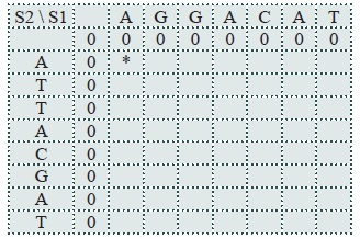
The first step in the Smith-Waterman method is to create a matrix (a table) T in which there are len(S1+1) columns and len(S2+1) rows. The first index in T(i,j) refers to the column and the second index is the row. The values in the current row are a function of those in the previous one. Place a 0 in each element of the first row and the first column. For the two strings used previously this would look like the table below.
Now, for any element T(i,j) the neighboring elements are:
T(i - 1, j - 1) T(i, j - 1) T(i + 1, j - 1)
T(i - 1, j) T(i, j) T(i + 1, j)
The first cell to fill in the table T is T(1,1), marked with a “*” character in the example to the left. The relation used to fill this cell has four parts:
1. T (i – 1, j –1) + σ (S1(i), S2( j)) The characters in the row and column match, so σ(S1(i), S2( j)) = σ (A, A) =1+ T(0,0) = 2
2. Gap penalty is -1, T(i-1, j) = 0, T(0, 1) = 0. Result is -1
3. Gap penalty is -1, T(i, j-1) = T(1,1) = 0. Result is -1
4. Result is 0
The maximum value of these four calculations is 1, so T(1, 1) = 2.
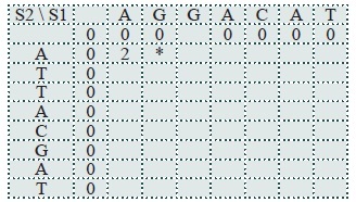
The next cell to compute is T(2,1). This time the two characters are not the same, so:
1. T (i −1, j −1) + σ (S1(i), S2( j))where σ (S1(i), S2( j)) = σ (G, A) = −1+ T(1,0) =
2. Gap penalty is -1, T(i - 1,j) = T(1,1) = 2.
Result is 2 - 1 = 1
3. Gap penalty is -1, T(i, j-1) = T(2,1) = 0. Result is -1
and so T(2,1) = 1
For T(3,1):
1. G and A are not the same, s(G, T) = -2:
2. T(i - 1.j) = T(2,1) = 1 so 1-1 = 0
3. T(i, j - 1) = T(3,0) = 0 so 0 – 1 = -1
4. 0
Result is 0
For T(4,1):
1. σ (A, A) = 2,
2. T(i - 1, j) = T(3, 1) = 0, 0-gap = -1
3. T(i, j -1) = T(4, 0) =0, 0-gap = -1
4. 0
Result is 2
For T(5, 1):
1. σ (C, A) = -2,
2. T(i - 1, j) = T(4, 1) = 2, 2-gap = 1
3. T(i, j - 1) = T(5, 0) =0, 0-gap = -1
4. 0
Result is 1
For T(6, 1):
1. σ (A,A) = 2,
2. T(i - 1, j) = T(5, 1) = 1, 1-gap = 0
3. T(i, j - 1) = T(6 0) =0, 0-gap = -1
4. 0
Result is 2
Finally for T(7,1):
1. σ (T, A) = -2,
2. T(i - 1, j) = T(6, 1) = 2, 2-gap = 1
3. T(i, j - 1) = T(7 0) =0, 0-gap = -1
4. 0
Result is 1
The result after row 2 is complete is:

Now move to the next row. The process repeats until all cells have been examined and assigned values. For this example the final matrix is:
The lower right entry is column 7 row 8, or (7,8).
This matrix indicates the degree of match at points in the string. To determine the actual match between the strings, begin with the largest value in the matrix. In this case it is in the lower right corner, but that’s not always true. Wherever the maximum is, start at that point in the matrix and trace left and upwards; this is essentially moving from the end of each string back to the beginning. At each step the move is left, up, or diagonally.
The process will build two ways to match the string. One indicates how to change s1 into s2 (call this M1), and the other indicates how to turn s2 into s1 (call this M2). Both strings are constructed from, in this case, (7,9) back
to (0,0).
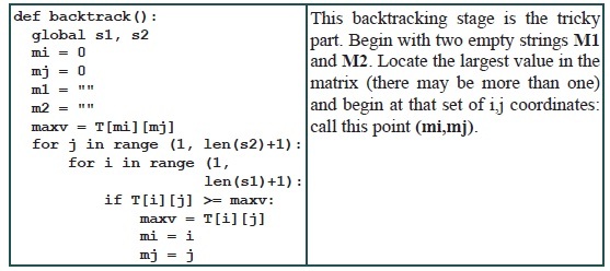
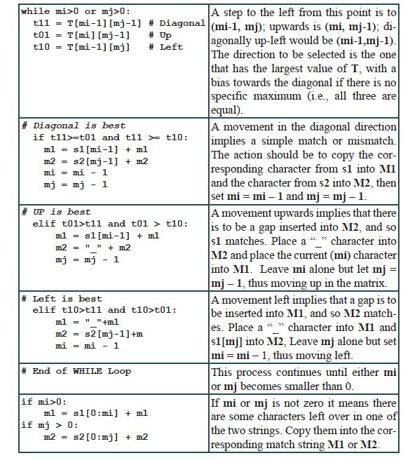
If there is more than one cell in T with a maximum value, then a route should be traced back from each maximum.
For the example string the result is:
M1 = AGGACCAT
M2 = ATTAC_AT
There is a mismatch at the GG/TT pair and an inserted gap in M2.
11.6 SUMMARY
A discussion of some of the more important problem types studied by scientists was presented along with some method for their solution. The root of an equation is the place where its value is zero, and Newton’s method was described as a means of finding a root. Newton’s method requires that the derivative of the function be known, so means of numerically determining the derivative were also discussed.
Since derivatives could be calculated, methods for performing integration were described and functions for doing the calculation using the trapezoidal rule were written.
One of the more common calculations in science is to find an optimum value for a function. Another method of Newton’s was used to find maxima or minima of a function.
The modeling of data is important in scientific (and other) disciplines. A method for finding the best straight line that passes through a set of data was illustrated (linear regression) and code was designed and tested for this problem.
Evolutionary algorithms can be used to find the optimum of a function, and is especially useful when dealing with multidimensional functions or functions that have many local optima, and when no derivative of the function exists.
Biologists sometimes need to match sequences of DNA. A method that does this using bases as characters and sequences as strings was presented; this is the Smith-Waterman algorithm for local sequence matching, and is commonly used for these problems.
Exercises
1. Modify the root finding example so that a numerical derivative is used instead of an analytical one (i.e., use derive1() or derive2()). This is a more practical situation. What is the effect?
2. Modify the trap0() function in the trapezoid rule example so that it never calls the function being evaluated more than once for any point.
3. Look up Simpson’s Rule and code your own version. Compare it with the trapezoid rule for two functions of your choice. Which one is more accurate after each iteration?
4. Write a function error() that accepts X and Y data tuples, and values a and b. It returns the total error between the data points and the curve ax2+bx.
5. The (natural) logarithm of a value v is defined to be the integral of 1/x from 1 to v. Create a function that calculates the natural log using the existing integration function.
6. Run the evolutionary algorithm to optimize the Goldstein-Price twenty times. Does it ever fail to approach the minimum? How often? What can be done if an EA does not arrive at an optimum, and how can it be determined?
7. Using software developed in this chapter, find two positive numbers whose sum is 9 and so that the product of one number and the square of the other number is a maximum.
Notes and Other Resources
Online edit distance calculator: http://planetcalc.com/1721/
Smith-Waterman algorithm: http://www.slideshare.net/avrilcoghlan/the-smith-waterman-algorithm
https://www.youtube.com/watch?v=jrJ23aaByE8
1. D. Levy. Lecture Notes, (Ch 5) Numerical Differentiation, http://www2.math.umd.edu/~dlevy/classes/amsc466/lecture-notes/differentiation-chap.pdf
2. William Press, Saul Teukolsky, William Vetterling, and Brian Flannery. (2007). Numerical Recipes: The Art of Scientific Computation, 3rd edition, Cambridge University Press.
3. Richard Hamming. (1987). Numerical Methods for Scientists and Engineers, Dover Publications.
4. J. R. Parker. (2002). Genetic Algorithms for Continuous Problems, 15th Canadian Conference on Artificial Intelligence, Calgary, Alberta,
May 27–29.
5. D. E. Goldberg. (1989). Genetic Algorithms, Optimization, and Machine Learning, Addison-Wesley, Reading, MA.
6. vlab.amrita.edu. (2012). Global Alignment of Two Sequences - Needleman-Wunsch Algorithm, Retrieved 9 December 2015, vlab.amrita.edu/?sub=3&brch=274&sim=1431&cnt=1
7. S. B. Needleman and C. D. Wunsch. (1970). A general method applicable to the search for similarities in the amino acid sequence of two proteins,
J. Mol. Biol., 48, 443–453.
8. T. F. Smith and M. S. Waterman. (1981). Identification of common molecular subsequences, J. Mol. Biol., 147(1), 195-197.