Chapter 2

Saving Time with Function Tools

IN THIS CHAPTER

Displaying the Insert Function dialog box

Finding the function you need

Using the Function Arguments dialog box

Entering formulas and functions

Excel has so many functions that it’s both a blessing and a curse. You can do many things with Excel functions — if you can remember them all! Even if you remember many function names, memorizing all the arguments the functions can use is a challenge.

Arguments are pieces of information that functions use to calculate and return a value.

Never fear: Microsoft hasn’t left you in the dark with figuring out which arguments to use. Excel has a great utility to help you insert functions, and their arguments, into your worksheet. This makes it a snap to find and use the functions you need. You can save both time and headaches, and make fewer errors to boot — so read on!

Getting Familiar with the Insert Function Dialog Box

The Insert Function dialog box (shown in Figure 2-1) is designed to simplify the task of using functions in your worksheet. The dialog box not only helps you locate the proper function for the task at hand, but also provides information about the arguments that the function takes. If you use the Insert Function dialog box, you don’t have to type functions directly in worksheet cells. Instead, the dialog box guides you through a (mostly) point-and-click procedure — a good thing, because if you’re anything like me, you need all the help you can get.

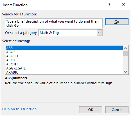
FIGURE 2-1: Use the Insert Function dialog box to easily enter functions in a worksheet.

In the Insert Function dialog box, you can browse functions by category or scroll the complete alphabetical list. A search feature — you type a word or phrase in the Search for a Function box, click the Go button, and see what comes up — is helpful. When you highlight a function in the Select a Function box, a brief description of what the function does appears under the list. You can also click the Help on This Function link at the bottom of the dialog box to view more detailed information about the function.

You can display the Insert Function dialog box in three ways:

• Click the Insert Function button on the Formulas tab.
• On the Formula Bar, click the smaller Insert Function button (which looks like f_x).
• Click the small arrow to the right of the AutoSum feature on the Formulas tab, and select More Functions (see Figure 2-2). AutoSum has a list of commonly used functions that you can insert with a click. If you select More Functions, the Insert Function dialog box opens.

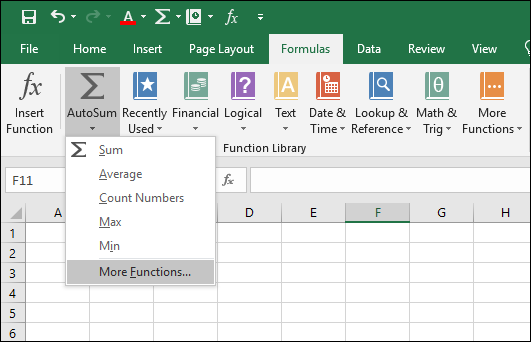
FIGURE 2-2: The AutoSum button offers quick access to basic functions and the Insert Function dialog box.

Finding the Correct Function

The first step in using a function is finding the one you need! Even when you do know the one you need, you may not remember all the arguments it takes. You can find a function in the Insert Function dialog box in two ways:

• Search: Type one or more keywords or a phrase in the Search for a Function box, then click the Go button.
  • If a match is made, the Or Select a Category drop-down menu displays Recommended, and the Select a Function box displays a list of the functions that match your search.
  • If no match is made, the Or Select a Category drop-down menu displays Most Recently Used functions, and the most recently used functions appear in the Select a Function dialog box. The Search for a Function box displays a message to rephrase the text entered for the search.
• Browse: Click the Or Select a Category down arrow, and from the drop-down menu, select All or an actual function category. When an actual category is selected, the Select a Function box updates to show just the relevant functions. You can look through the list to find the function you want. Alternatively, if you know the category, you can select it on the Formulas tab.

Table 2-1 lists the categories in the Or Select a Category drop-down menu. Finding the function you need is different from knowing which function you need. Excel is great at giving you the functions, but you do need to know what to ask for.

TABLE 2-1 Function Categories in the Insert Function Dialog Box

Category	Type of Functions
Most Recently Used	The last several functions you used.
All	The entire function list, sorted alphabetically.
Financial	Functions for managing loans, analyzing investments, and so on.
Date & Time	Functions for calculating days of the week, elapsed time, and so on.
Math & Trig	A considerable number of mathematical functions.
Statistical	Functions for using descriptive and inferential statistics.
Lookup & Reference	Functions for obtaining facts about and data on worksheets.
Database	Functions for selecting data in structured rows and columns.
Text	Functions for manipulating and searching text values.
Logical	Boolean functions (AND, OR, and so on).
Information	Functions for getting facts about worksheet cells and the data therein.
Web	A few functions that are useful when sharing data with web services.
Engineering	Engineering and some conversion functions. These functions are also provided in the Analysis ToolPak.
Cube	Functions used with online analytical processing (OLAP) cubes.
Compatibility	Some functions were updated as of Excel 2010 and Excel 2013. The functions in this category are the older versions that remain compatible with Excel 2007 and earlier versions.
User Defined	Any available custom functions created in VBA code or from add-ins. This category may not be listed.

Entering Functions Using the Insert Function Dialog Box

Now that you’ve seen how to search for or select a function, it’s time to use the Insert Function dialog box to actually insert a function. The dialog box makes it easy to enter functions that take no arguments and functions that do take arguments. Either way, the dialog box guides you through the process of entering the function.

Sometimes, function arguments are not values, but references to cells, ranges, named areas, or tables. That this is also handled in the Insert Function dialog box makes its use so beneficial.

Selecting a function that takes no arguments

Some functions return a value, period. No arguments are needed for these functions. This means you don’t have to have some arguments ready to go. What could be easier? Here’s how to enter a function that does not take any arguments. The TODAY function is used in this example:

1. Position the cursor in the cell where you want the results to appear.
2. Click the Insert Function button on the Formulas tab to open the Insert Function dialog box.
3. Select All in the Or Select a Category drop-down menu.

4. Scroll through the Select a Function list until you see the TODAY function, and click it.

   Figure 2-3 shows what the screen looks like.

5. Click OK.

   The Insert Function dialog box closes, and the Function Arguments dialog box opens. The dialog box tells you that function does not take any arguments. Figure 2-4 shows how the screen looks now.

6. Click OK.

   Doing this closes the Function Arguments dialog box, and the function entry is complete.

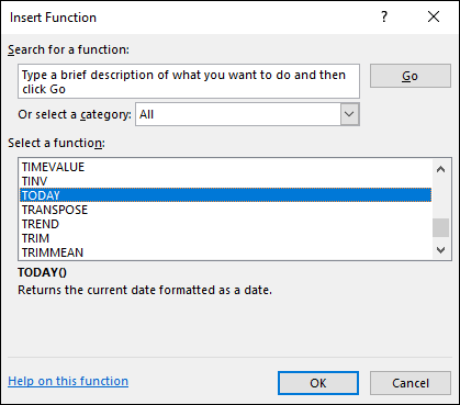
FIGURE 2-3: Selecting a function.

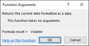
FIGURE 2-4: Confirming that no arguments exist with the Function Arguments dialog box.

You may have noticed that the Function Arguments dialog box says that the Formula result will equal Volatile. This is nothing to be alarmed about! This just means the answer can be different each time you use the function. For example, TODAY will return a different date when used tomorrow.

Figure 2-5 shows how the function’s result has been returned to the worksheet. Cell B2 displays the date when I wrote this example. The date you see on your screen is the current date.

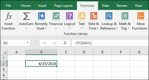
FIGURE 2-5: Populating a worksheet cell with today’s date.

Most functions do take arguments. The few that do not take arguments can return a result without needing any information. For example, the TODAY function just returns the current date. It doesn’t need any information to figure this out.

Selecting a function that uses arguments

Most functions take arguments to provide the information that the functions need to perform their calculations. Some functions use a single argument; others use many. Taking arguments and using arguments are interchangeable terms. Most functions take arguments, but the number of arguments depends on the actual function. Some functions take a single argument, and some can take up to 255.

The following example shows how to use the Insert Function dialog box to enter a function that does use arguments. The example uses the PRODUCT function. Here’s how to enter the function and its arguments:

1. Position the cursor in the cell where you want the results to appear.

2. Click the Insert Function button on the Formulas tab.

   Doing this opens the Insert Function dialog box.

3. Select Math & Trig in the Or Select a Category drop-down menu.

4. Scroll through the Select a Function list until you see the PRODUCT function and then click it.

   Figure 2-6 shows what the screen looks like.

5. Click OK.

   The Insert Function dialog box closes, and the Function Arguments dialog box opens. Figure 2-7 shows what the screen looks like. The dialog box tells you that this function can take up to 255 arguments, yet there appears to be room for only 2. As you enter arguments, the dialog box provides a scroll bar to manage multiple arguments.

6. In the Function Arguments dialog box, enter a number in the Number1 box.

7. Enter another number in the Number2 box.

   You are entering actual arguments. As you enter numbers in the dialog box, a scroll bar appears, letting you add arguments. Enter as many as you like, up to 255. Figure 2-8 shows how I entered eight arguments. Also look at the bottom left of the dialog box. As you enter functions, the formula result is instantly calculated. Wouldn’t it be nice to be that smart?

8. Click OK to complete the function entry.

   Figure 2-9 shows the worksheet’s result.

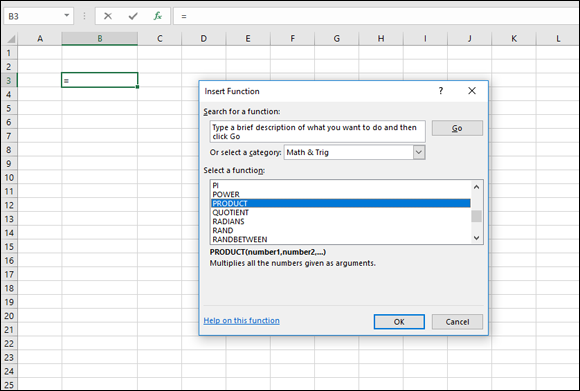
FIGURE 2-6: Preparing to multiply some numbers with the PRODUCT function.

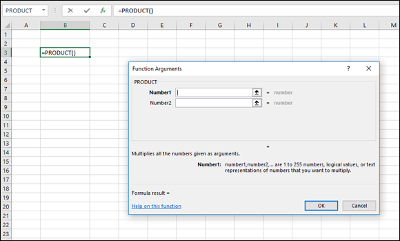
FIGURE 2-7: Ready to input function arguments.

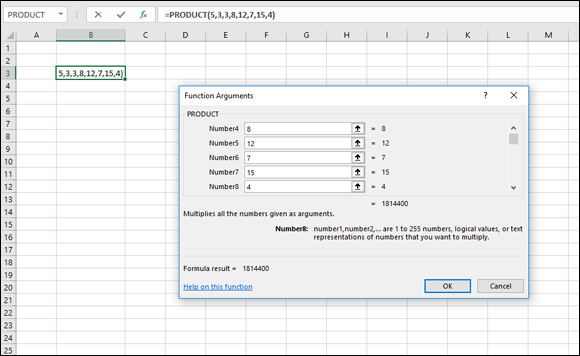
FIGURE 2-8: Getting instant results in the Function Arguments dialog box.

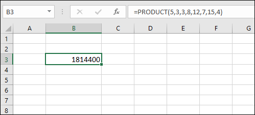
FIGURE 2-9: Getting the final answer from the function.

Entering cells, ranges, named areas, and tables as function arguments

Excel is so cool. You can not only provide single cell references as arguments, but also, in many cases you can enter an entire range reference, or the name of an area or table, as a single argument! What’s more, you can enter these arguments by using either the keyboard or the mouse.

This example demonstrates using both single cell and range references as well as a named area and table as arguments. For this example, I use the SUM function. Here’s how to use the Insert Function dialog box to enter the function and its arguments:

1. Enter some numbers in a worksheet in contiguous cells.

2. Select the cells and then click the Table button on the Insert tab.

   The Create Table dialog box opens.

3. Click OK to complete making the table.

   The Ribbon should display table style and other options. (If not, look along the Excel title bar for Table Tools, and click it.) On the left end of the Ribbon is the name that Excel gave the table. You can change the name of the table, as well as the appearance. Jot down the name of the table. You need to re-enter the table name further in these steps.

4. Somewhere else on the worksheet, enter numbers in contiguous cells.

5. Select the cells and then click the Define Name button on the Formulas tab.

   The New Name dialog box opens.

6. Enter a name for the area.

   I used the name MyArea. See Figure 2-10 to see how the worksheet is shaping up.

7. Enter some more numbers in contiguous cells, either across a row or down a column.
8. Enter a single number in cell A1.
9. Click an empty cell where you want the result to appear.

10. Click the Insert Function button on the Formulas tab.

    The Insert Function dialog box opens.

11. Select the SUM function.

    SUM is in the All or Math & Trig category, and possibly in the Recently Used category.

12. Click OK.

    The Function Arguments dialog box opens.

    To the right of each Number box is a small fancy button — a special Excel control sometimes called the RefEdit. It allows you to leave the dialog box, select a cell or range on the worksheet, and then go back to the dialog box. Whatever cell or range you click or drag over on the worksheet is brought into the entry box as a reference.

    You can type cell and range references, named areas, and table names directly in the Number boxes as well. You can also click directly on cells or ranges on the worksheet. The RefEdit controls are there to use if you want to work with the mouse instead.

13. Click the first RefEdit.

    The dialog box shrinks so that the only thing visible is the field where you enter data. Click cell A1, where you entered a number.

14. Press Enter.

    The Function Arguments dialog box reappears.

15. In the second entry box, type the name of your named area.

    If you don’t remember the name you used, use the RefEdit control to select the area on the worksheet.

16. In the third entry box, enter your table name and press Enter.
17. If you don’t remember the name you used, use the RefEdit control to select the table.

18. In the fourth entry box, enter a range from the worksheet where some values are located.

    It does not matter if this range is part of a named area or table. Use the RefEdit control if you want to just drag the mouse over a range of numbers. Your screen should look similar to Figure 2-11.

19. Click OK.

    The final sum from the various parts of the worksheet displays in the cell where the function was entered. Figure 2-12 shows how the example worksheet turned out.

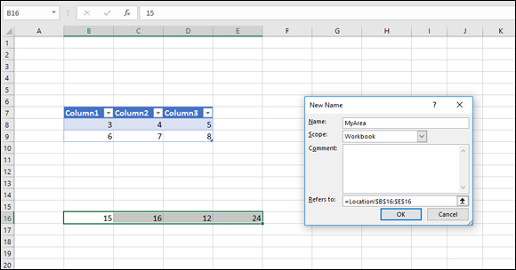
FIGURE 2-10: Adding a table and a named area to a worksheet.

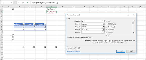
FIGURE 2-11: Entering arguments.

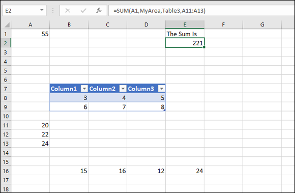
FIGURE 2-12: Calculating a sum based on cell and range references.

Congratulations! You did it. You successfully inserted a function that took a cell reference, a range reference, a named area, and a table name. You’re harnessing the power of Excel. Look at the result — the sum of many numbers located in various parts of the worksheet. Just imagine how much summing you can do. You can have up to 255 inputs, and if necessary, each one can be a range of cells.

You can use the Insert Function dialog box at any time while entering a formula. This is helpful when the formula uses some values and references in addition to a function. Just open the Insert Function dialog box when the formula entry is at the point where the function goes.

Getting help in the Insert Function dialog box

The number of functions and their exhaustive capabilities give you the power to do great things in Excel. However, from time to time, you may need guidance on how to get functions to work. Luckily for you, help is just a click away.

Both the Insert Function and Function Arguments dialog boxes have a link to the Help system. At any time, you can click the Help on This Function link in the lower-left corner of the dialog box and get help on the function you’re using. The Help system has many examples. Often, reviewing how a function works leads you to other, similar functions that may be better suited to your situation.

Using the Function Arguments dialog box to edit functions

Excel makes entering functions with the Insert Function dialog box easy. But what do you do when you need to change a function that has already been entered in a cell? What about adding arguments or taking some away? There is an easy way to do this! Follow these steps:

1. Click the cell with the existing function.

2. Click the Insert Function button.

   The Function Argument dialog box appears. This dialog box is already set to work with your function. In fact, the arguments that have already been entered in the function are displayed in the dialog box as well!

3. Add, edit, or delete arguments, as follows:
   • To add an argument (if the function allows), use the RefEdit control to pick up the extra values from the worksheet. Alternatively, if you click the bottom argument reference, a new box opens below it, and you can enter a value or range in that box.
   • To edit an argument, simply click it and change it.
   • To delete an argument, click it and press the Backspace key.

4. Click OK when you’re finished.

   The function is updated with your changes.

Directly Entering Formulas and Functions

As you get sharp with functions, you will likely bypass the Insert Function dialog box altogether and enter functions directly. One place you can do this is in the Formula Bar. Another way is to just type in a cell.

Entering formulas and functions in the Formula Bar

When you place your entry in the Formula Bar, the entry is really going into the active cell. However, because the active cell can be anywhere, you may prefer entering formulas and functions directly in the Formula Bar. That way, you know that the entry will land where you need it. Before you enter a formula in the Formula Box (on the right end of the Formula Bar), the Name Box on the left lets you know where the entry will end up. The cell receiving the entry may be not be in the visible area of the worksheet. Gosh, it could be a million rows down and thousands of columns to the right! After you start entering the formula, the Name Box becomes a drop-down menu of functions. This menu is useful for nesting functions. As you enter a function in the Formula Box, you can click a function in the Name Box, and the function is inserted into the entry you started in the Formula Box. Confused? Imagine what I went through explaining that! Seriously, though, this is a helpful way to assemble nested functions. Try it, and get used to it; it will add to your Excel smarts.

When your entry is finished, press Enter or click the little check-mark Enter button to the left of the Formula Box.

Figure 2-13 makes this clear. A formula is being entered in the Formula Box, and the Name Box follows along with the function(s) being entered. Note, though, that the active cell is not in the viewable area of the worksheet. It must be below and/or to the right of the viewable area because the top-left portion of the worksheet is shown in Figure 2-13.

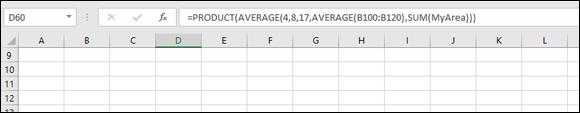
FIGURE 2-13: Entering a formula in the Formula Box has its conveniences.

In between the Name Box and the Formula Box are three small buttons. From left to right, they do the following:

• Cancel the entry.
• Complete the entry.
• Display the Insert Function dialog box.

The Cancel and Enter Function buttons are enabled only when you enter a formula, a function, or just plain old values on the Formula Bar or directly in a cell.

Entering formulas and functions directly in worksheet cells

Perhaps the easiest entry method is typing the formula directly in a cell. Just type formulas that contain no functions and press Enter to complete the entry. Try this simple example:

1. Click a cell where the formula is to be entered.

2. Enter this simple math-based formula:

   =6 + (9/5) *100

3. Press Enter.

   The answer is 186. (Don’t forget the order of operators; see Chapter 18 for more information about the order of mathematical operators.)

Excel makes entering functions in your formulas as easy as a click. As you type the first letter of a function in a cell, a list of functions starting with that letter is listed immediately (see Figure 2-14).

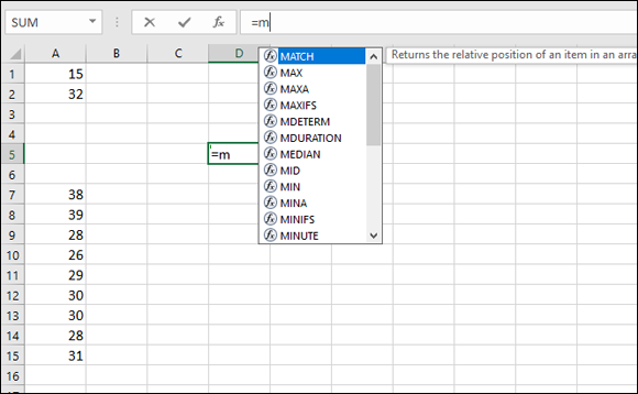
FIGURE 2-14: Entering functions has never been this easy.

The desired function in this example is MIN, which returns the minimum value from a group of values. As soon as you type M (first enter the equal sign if this is the start of a formula entry), the list in Figure 2-14 appears, showing all the M functions. Now that an option exists, either keep typing the full function name, or scroll to MIN and press the Tab key. Figure 2-15 shows just what happens when you do the latter. MIN is completed and provides the required syntax structure — not much thinking involved! Now your brain can concentrate on more interesting things, such as poker odds. (Will Microsoft ever create a function category for calculating poker odds? Please?) In Figure 2-15, the MIN function is used to find the minimum value in the range A7:A15 (which is multiplied with the sum of the values in A1 plus A2). Entering the closing parenthesis and then pressing Enter completes the function. In this example, the answer is 1222.

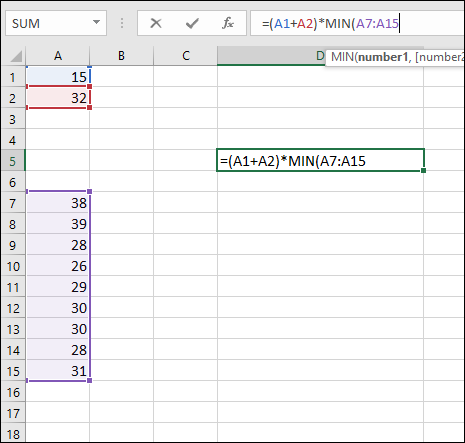
FIGURE 2-15: Completing the direct-in-the-cell formula entry.

A1: 15

A2: 32

A7: 38

A8: 39

A9: 28

A10: 26

A11: 29

A12: 30

A13: 30

A14: 28

A15: 31

The formula in D5 is =(A1+A2) * MIN(A7:A15).

Excel’s capability to show a list of functions based on spelling is called Formula AutoComplete.

You can turn Formula AutoComplete on or off in the Excel Options dialog box by following these steps:

1. Click the File tab at the top left of the screen.
2. Click Options.
3. In the Excel Options dialog box, select the Formulas tab.
4. In the Working with Formulas section, select or deselect the Formula AutoComplete check box. See Figure 2-16.
5. Click OK.

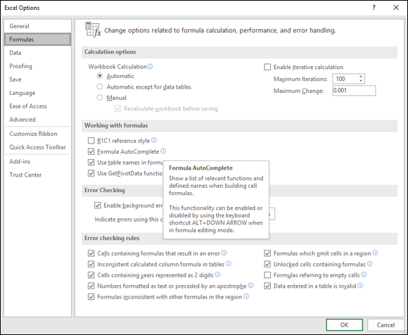
FIGURE 2-16: Setting Formula AutoComplete.