Chapter 15

Digging Up the Facts

IN THIS CHAPTER

Getting information about a cell or range

Finding out about Excel or your computer system

Testing for numbers, text, and errors

In this chapter, I show you how to use Excel’s information functions, which you use to obtain information about cells, ranges, and the workbook you’re working in. You can even get information about the computer you’re using. What will they think of next?

The information functions are great for getting formulas to focus on just the data that matter. Some functions even help shield you from Excel’s confusing error messages. The first time I saw the #NAME? error, I thought Excel was asking me to enter a name (just another of the more exciting Excel moments). Now at least I know to use the ISERROR or ERROR.TYPE functions to make error messages more meaningful. And after reading this chapter, so will you!

Getting Informed with the CELL Function

The CELL function provides feedback about cells and ranges in a worksheet. You can find out what row and column a cell is in, what type of formatting it has, whether it's protected, and so on.

CELL takes two arguments:

• The first argument, which is enclosed in double quotes, tells the function what kind of information to return.
• The second argument tells the function which cell or range to evaluate. If you specify a range that contains more than one cell, the function returns information about the top-left cell in the range. The second argument is optional; when it isn’t provided, Excel reports back on the most recently changed cell.

Table 15-1 shows the list of possible entries for the first argument of the CELL function.

TABLE 15-1 Selecting the First Argument for the CELL Function

Argument	Example	Comment
address	=CELL("address")	Returns the address of the last changed cell.
col	=CELL("col",Sales)	Returns the column number of the first cell in the Sales range.
color	=CELL("color",B3)	Tells whether a particular cell (in this case, cell B3) is formatted in such a way that negative numbers are represented in color. The number, currency, and custom formats have selections for displaying negative numbers in red. If the cell is formatted for color-negative numbers, a 1 is returned; otherwise, a 0 is returned.
contents	=CELL("contents",B3)	Returns the contents of a particular cell (in this case, cell B3). If the cell contains a formula, returns the result of the formula and not the formula itself.
filename	=CELL("filename")	Returns the path, filename, and worksheet name of the workbook and worksheet that has the CELL function in it (for example, C:\Customers\[Acme Company]Sheet1). The function results in a blank answer in a new workbook that has not yet been saved.
format	=CELL("format",D12)	Returns a cell’s number format (in this case, cell D12). See Table 15-2 for a list of possible returned values.
parentheses	=CELL("parentheses",D12)	Returns 1 if a cell (in this case, D12) is formatted to have either positive values or all values displayed with parentheses. Otherwise, 0 is returned. A custom format is needed to make parentheses appear with positive values in the first place.
prefix	=CELL("prefix",R25)	Returns the type of text alignment in a cell (in this case, cell R25). There are a few possibilities: a single quotation mark (‘) if the cell is left-aligned; a double quotation mark (") if the cell is right-aligned; a caret (^) if the cell is set to centered; or a backslash (\) if the cell is fill-aligned. If the cell being evaluated is blank or has a number, the function returns nothing.
protect	=CELL("protect",D12)	Returns 1 if a cell’s protection (in this case, cell D12) is set to locked; otherwise, a 0 is returned. The returned value is not affected by whether the worksheet is currently protected.
row	=CELL("row",Sales)	Returns the row number of the first cell in the Sales range.
type	=CELL("type",D12)	Returns a value corresponding to the type of information in a cell (in this case, cell D12). There are three possible values: b if the cell is blank; l if the cell has alphanumeric data; and v for all other possible values, including numbers and errors.
width	=CELL("width")	Returns the width of the last changed cell, rounded to an integer. For example, a width of 18.3 is returned as 18.

The second argument, whether it’s there or not, plays a key role in how the CELL function works. When it’s included, the second argument is a cell address, such as B12, or a range name, such as Sales. Of course, you could have a range that is only one cell, but I won’t confuse the issue!

If you enter a nonexistent range name for the second argument, Excel returns the #NAME? error. Excel can’t return information about something that doesn’t exist!

An interesting way to use CELL is to keep track of the last entry on a worksheet. Say you’re updating a list of values. The phone rings, and you’re tied up for a while on the call. When you get back to your list, you’ve forgotten where you left off. Yikes! What a time to think “If only I had used the CELL function!”

Figure 15-1 shows such a worksheet. Cell B18 displays the address of the last cell that was changed.

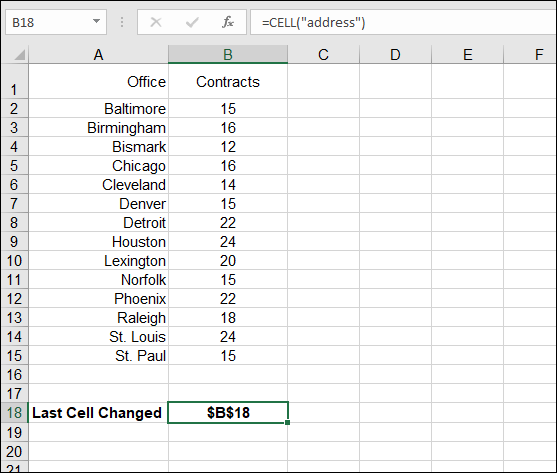
FIGURE 15-1: Keeping track of which cell had the latest entry.

Using CELL with the filename argument is great for displaying the workbook’s path. This technique is common for printed worksheet reports. Being able to find the workbook file that a report was printed from 6 months ago is a real time-saver. Don’t you just love it when the boss gives you an hour to create a report, doesn’t look at it for 6 months, and then wants to make a change? Here’s how you enter the CELL function to return the filename:

=CELL("filename")

You can format cells in many ways. When the first argument of CELL is format, a code is returned that corresponds to the formatting. The possible formats are those listed in the Format Cells dialog box. Table 15-2 shows the formats and the code that CELL returns.

TABLE 15-2 Returned Values for the format Argument

Format	Returned Value from CELL Function
General	G
0	F0
#,##0	,0
0.00	F2
#,##0.00	,2
$#,##0_);($#,##0)	C0
$#,##0_);[Red]($#,##0)	C0-
$#,##0.00_);($#,##0.00)	C2
$#,##0.00_);[Red]($#,##0.00)	C2-
0%	P0
0.00%	P2
0.00E+00	S2
# ?/? or ??/??	G
m/d/yy or m/d/yy h:mm or mm/dd/yy	D4
d-mmm-yy or dd-mmmm-yy	D1
d-mmm or dd-mmm	D2
mmm-yy	D3
mm/dd	D5
h:mm AM/PM	D7
h:mm:ss AM/PM	D6
h:mm	D9
h:mm:ss	D8

Using CELL with the format argument lets you add a bit of smarts to your worksheet. Figure 15-2 shows an example of CELL making sure information is correctly understood. The dates in column A are of the d-mmm format. The downside of this format is that the year is not known. So cell A1 has been given a formula that uses CELL to test the dates' format. If the d-mmm format is found in the first date (in cell A4), cell A1 displays a message that includes the year from cell A4. After all, cell A4 has a year; it’s just formatted not to show it. This way, the year is always present — either in the dates themselves or at the top of the worksheet.

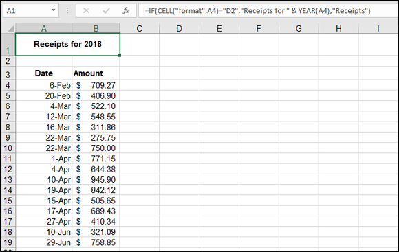
FIGURE 15-2: Using CELL and the format argument to display a useful message.

The formula in cell A1 — =IF(CELL("format",A4)="D2","Receipts for "&YEAR(A4),"Receipts") — says that if the formatting in A4 is d-mmm (according to the values in Table 15-2), display the message with the year; otherwise, just display Receipts.

Here's how to use the CELL function:

1. Position the cursor in the cell where you want the results to appear.
2. Type =CELL( to begin the function entry.

3. Enter one of the first argument choices listed in Table 15-1.

   Make sure to surround it with double quotes (" ").

4. If you want to tell the function which cell or range to use, type a comma (,).
5. If you want, enter a cell address or the name of a range.
6. Type a ) and press Enter.

Getting Information About Excel and Your Computer System

Excel provides the INFO function to get information about your computer and about the program itself. INFO takes a single argument that tells the function what type of information to return. Table 15-3 shows how to use the INFO function.

TABLE 15-3 Using INFO to Find Out About Your Computer or Excel

Argument	Example	Comment
directory	=INFO("directory")	Returns the path of the current directory. Note that this is not necessarily the same path of the open workbook.
numfile	=INFO("numfile")	Returns the number of worksheets in all open workbooks. The function includes worksheets of add-ins, so the number could be misleading.
origin	=INFO("origin")	Returns the address of the cell at the top and to the left of the scrollable area. An A$ prefix in front of the cell address is for compatibility with Lotus 1-2-3.
osversion	=INFO("osversion")	Returns the name of the current operating system.
recalc	=INFO("recalc")	Returns the status of the recalculation mode: Automatic or Manual.
release	=INFO("release")	Returns the version number of Excel being run.
system	=INFO("system")	Returns the name of the operating environment: mac or pcdos.

One useful application of the INFO function is to use the returned Excel version number to determine whether the workbook can use a newer feature. For example, the ability to work with XML data has been available only in Excel 2002 and later. By testing the version number, you can be notified whether you can work with XML data. This formula uses the release choice as the argument:

=IF(INFO("release")>9,"This version can import XML", "This version cannot import XML")

Figure 15-3 shows values returned with the INFO function.

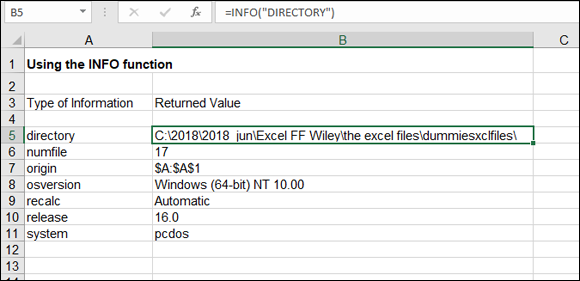
FIGURE 15-3: Getting facts about the computer with the INFO function.

Here’s how to use the INFO function:

1. Position the cursor in the cell where you want the results to appear.
2. Type =INFO( to begin the function entry.

3. Enter one of the argument choices listed in Table 15-3.

   Make sure to surround it with double quotes (" ").

4. Type a ) and press Enter.

Finding What IS and What IS Not

A handful of IS functions report back a true or false answer about certain cell characteristics. For example, is a cell blank, or does it contain text? These functions are often used in combination with other functions — typically, the IF function — to handle errors or other unexpected or undesirable results.

The errors Excel reports are not very friendly. What on earth does #N/A really tell you? The functions I describe in this section don't make the error any clearer, but they give you a way to instead display a friendly message like “Something is wrong, but I don’t know what it is.”

Table 15-4 shows the IS functions and how they’re used. They all return either True or False, so the table just lists them.

TABLE 15-4 Using the IS Functions to See What Really Is

Function	Comment
=ISBLANK(value)	Tells whether a cell is blank.
=ISERR(value)	Tells whether a cell contains any error other than #N/A.
=ISERROR(value)	Tells whether a cell contains any error.
=ISEVEN(value)	Tells whether a number is even.
=ISFORMULA	Tells whether the cell contains a formula.
=ISLOGICAL(value)	Tells whether the value is logical.
=ISNA(value)	Tells whether a cell contains the #N/A error.
=ISNONTEXT(value)	Tells whether a cell contains a number or error.
=ISNUMBER(value)	Tells whether a cell contains a number.
=ISODD(value)	Tells whether a number is odd.
=ISOWEEKNUM	Tells the ISO week number for the entered date. (ISO is the International Organization for Standardization, a standards-setting consortium.)
=ISREF(value)	Tells whether the value is a reference.
=ISTEXT(value)	Tells whether a cell contains text.

ISERR, ISNA, and ISERROR

Three of the IS functions — ISERR, ISNA, and ISERROR — tell you about an error.

Error Function	Comments
ISERR	Returns true if the error is anything except the #N/A error. For example, the #DIV/0! error returns true.
ISNA	The opposite of ISERR. It returns true only if the error is #N/A.
ISERROR	Returns true for any type of error, including #N/A, #VALUE!, #REF!, DIV/0!, #NUM!, #NAME?, and #NULL!.

Why is #N/A treated separately? It is excluded from being handled with ISERR and has its own ISNA function. Actually, you can use #N/A to your advantage to avoid errors. How so? Figure 15-4 shows an example that calculates the percentage of surveys returned for some of Florida's larger cities. The calculation is simple: Just divide the returned number by the number sent.

FIGURE 15-4: Using an error to your advantage.

However, errors do creep in. For example, no surveys were sent to Gainesville, yet 99 came back. Interesting! The calculation becomes a division by zero error, which makes sense. On the other hand, Tallahassee had no surveys sent, but here, the returned value is the #N/A error, purposely entered. Next, look at column E. In this column, True or False is returned to indicate whether the calculation, per city, should be considered an error: Gainesville true, Tallahassee false.

The result true or false appears in column E because all the cells in column E use the ISERR function. The formula in cell E13, which tests the calculation for Tallahassee, is =ISERR(D13).

Simply put, D13 displays the #N/A error because its calculation (=C13/B13) uses a cell with an entered #N/A. The ISERR does not consider #N/A to be an error; therefore, E13 returns False. The upshot is that eyeballing column E makes it easy to distinguish entry and math errors from purposeful flagging of certain rows as having incomplete data.

ISBLANK, ISNONTEXT, ISTEXT, and ISNUMBER

The ISBLANK, ISNONTEXT, ISTEXT, and ISNUMBER functions tell you what type of data is in a cell.

Error Function	Comments
ISBLANK	Returns true if the cell is empty; otherwise, returns false.
ISNONTEXT	Returns true if the cell contains anything that is not text: a number, a date/time, or an error. The function returns true if the cell is blank or false if the cell contains text or a formula whose result is text.
ISTEXT	The opposite of ISNONTEXT: Returns true if the cell contains text or a formula whose result is text; otherwise, returns false.
ISNUMBER	Returns true if the cell contains a number or a formula whose result is a number; otherwise, returns false.

ISBLANK returns true when nothing is in a cell. Using ISBLANK is useful for counting how many cells in a range are blank. Perhaps you're responsible for making sure that 200 employees get their time sheets in every week. You can use a formula that lets you know how many employees have not yet handed in their hours.

Such a formula uses ISBLANK along with the IF and SUM functions, like this:

{=SUM(IF(ISBLANK(B5:B26),1,0))}

This formula makes use of an array. See Chapter 3 for more information on using array formulas. Figure 15-5 shows how this formula works. In columns A and B are lists of employees and their hours. The formula in cell A1 reports how many employees are missing their hours.

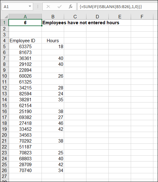
FIGURE 15-5: Calculating how many employees are missing an entry.

ISTEXT returns True when a cell contains any type of text. ISNONTEXT returns True when a cell contains anything that is not text, including numbers, dates, and times. The ISNONTEXT function also returns True if the cell contains an error.

The ISNUMBER function returns True when a cell contains a number, which can be an actual number or a number resulting from evaluation of a formula in the cell. You can use ISNUMBER as an aid to help data entry. Say you designed a worksheet that people fill out. One of the questions is age. Most people would enter a numeric value such as 18, 25, 70, and so on. But someone could type the age as text, such as eighteen, thirty-two, or “none of your business.” An adjacent cell could use ISNUMBER to return a message about entering the numeric age. The formula would look something like this:

=IF(ISNUMBER(B3),"","Please enter your age as a number")

Here's how to use any of the IS functions:

1. Position the cursor in the cell where you want the results to appear.

2. Enter one of the IS functions.

   For example, type =ISTEXT( to begin the function entry.

3. Enter a cell address.

4. Type a ) and press Enter.

   The result is always True or False.

Getting to Know Your Type

The TYPE function tells you what the type of the information is; for example:

• Number
• Text
• A logical value
• An error
• An array

In all cases TYPE returns a number:

• 1 is returned for numbers.
• 2 is returned for text.
• 4 is returned for logical values.
• 16 is returned for errors.
• 64 is returned for arrays.

Figure 15-6 shows each of these values returned by the TYPE function. Cells B3:B7 contain the TYPE function, with each row looking at the adjacent cell in column A. The returned value of 64 in cell B7 is a little different. This indicates an array as the type. The formula in cell B7 is =TYPE(A7:A9). This is an array of values from cells A7:A9.

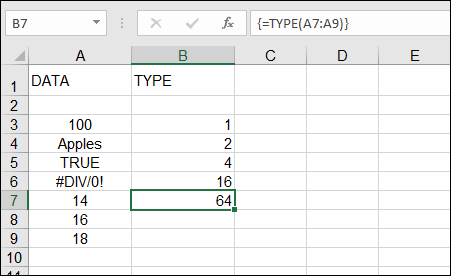
FIGURE 15-6: Getting the type of the data.

Here's how to use the TYPE function:

1. Position the cursor in the cell where you want the results to appear.
2. Enter =TYPE( to begin the function entry.
3. Enter a cell address or click a cell.
4. Type a ) and press Enter.

The ERROR.TYPE function returns a number that corresponds to the particular error in a cell. Table 15-5 shows the error types and the returned numbers.

TABLE 15-5 Getting a Number of an Error

Error Type	Returned Number
#NULL!	1
#DIV/0!	2
#VALUE!	3
#REF!	4
#NAME?	5
#NUM!	6
#N/A	7

The best thing about the ERROR.TYPE function is that you can use it to change those pesky errors to something readable! To do this, use the CHOOSE function along with ERROR.TYPE, like this:

=CHOOSE(ERROR.TYPE(H14),"Nothing here!","You can't divide by 0","A bad number has been entered", "The formula is referencing a bad cell or range","There is a problem with the entry","There is a problem with the entered value","Something is seriously wrong!")

See Chapter 14 for assistance on using the CHOOSE function. This is how you use the ERROR.TYPE function:

1. Position the cursor in the cell where you want the results to appear.
2. Enter =ERROR.TYPE( to begin the function entry.
3. Enter a cell address or click a cell.
4. Type a ) and press Enter.