1
Market Risk, Timing, and Formula Strategies
Whether you call it investing or playing the market, buying and selling stocks is risky business—risky but lucrative. In choosing to read this book, you have likely decided to build an investment portfolio that may include some of those risky stocks in order to garner some of those lucrative rewards. Before making investment decisions, you should have a reasonable idea of the typical risks you will face in the stock market and the likely rewards you might expect to earn. This chapter provides an introduction to these issues and familiarizes you with some historical data on market performance.
RISK AND MARKET RETURNS
First we will look at the investment returns that have been earned in the stock market in the past. Later in this section we discuss the risk inherent in these returns. Together, this information will provide you with a realistic sense of your opportunities in the stock market.
Market Returns over Time
When any wise market prognosticator is asked the inevitable question:
Is the stock market going to move up or down?, the unsatisfying but correct answer is:
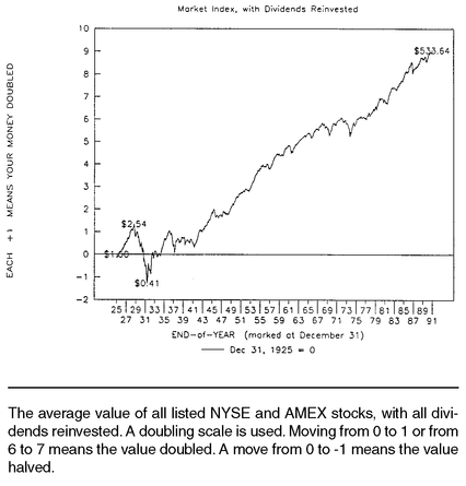
Yes, it will. Day-to-day movements are anyone’s guess, but over time the market has risen substantially. Stock price movements for the past 66 years are shown in
Figure 1-1.
1Note that a $1.00 investment on the last day of 1925 would have been worth $533.64 by the end of 1991. That’s a 9.98% compounded annual return over a period where inflation averaged 3.2%. Of course, you could have invested $2.54 prior to the October 1929 stock market crash and despaired as it went as low as $0.41 by mid-1932, losing over five-sixths of its value. Even though there has been only one such period in the past century, this scenario still highlights the magnitude of the potential risks faced when investing in the stock market.
If you (or more likely an ancestor) had invested $100 in the overall market each month during 1926-1991, your investment would have grown to $11,386,000, more than 140 times the total number of dollars you would have invested. Now admittedly, $100 a month was a lot of money back in the 1930s (worth about $800 in today’s dollars), but so is $11 million today. Let’s take a closer look at the type of risk entailed in attaining these investment rewards.
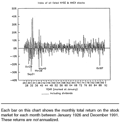
Figure 1-2 shows the total return (capital gains
plus dividends) for each individual month in the 66-year period. Although it is extremely unusual for the market to move more than 20% in a given month, you can see that it
has happened about ten times. The average market return for one month is slightly under +1.0% (0.95% monthly), or 12% annualized.
2 (See “Returns and Compounding” in the box on page 7.)
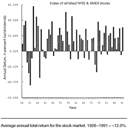
Figure 1-3 portrays similar data, but for years instead of months. Here it is easier to see that the market generally goes up, but that there is still random variability with no apparent pattern. The range of returns is from a − 44% loss to a +58% gain, although since World War II they fall in a tighter range of −28% to +51%. Individual stocks, of course, exhibit much more variability than the market as a whole, so avoid confusing
typical market returns with what might happen to a
single stock.

RETURNS and COMPOUNDING
A return on investment (e.g., 8%) must be connected with a period of time (e.g., a year). Annual terms are commonly used, but not always. When we shift our concern from one time period to a different one, we must “translate” the return figure as well.
Suppose the total return on a 2-year investment was 21%. A natural way of stating this would be to convert the 2-year return into an annual figure—a 1-year return. But simply dividing the 21% by 2, yielding an annual return figure of 10.50%, would be incorrect. Simple “averaging” of a return ignores compounding. Suppose you had a $100 two-year investment, and made a 10.50% return on it in the first year. That gives you $110.50. With another 10.50% return in the second year, you end up with $122.10 (10.50% of $110.50 is $11.60). This is a 2-year return of 22.10%, not just 21 %. Actually, a 21% two-year return is equivalent to a 10% annual return ($100 + 10% = $110; $110 + 10% = $121, a 21 % total return).
If
a is the annual return, then this formula will give you the compound return for
n-years:
(1 + a)n = 1 + n-year return
In the example above,
a =
10% and
n =
2, so:
(1 +
0.10)2 =
1.21 =
1 +
n-year return 0.21 =
21 % =
2-year return
The process works in reverse, too, to find the annual return given a longerperiod return. Taking the
n-th root (on a calculator, that’s raising something to the
1/n power), the formula is:
1 + a = n-th root(1 + n-year return)
or,
1 + a = (1 + n-year return)1/n
EXAMPLE: What annual rate gets you a 50% return over five years?
1 + a = 5-th root(1 + 0.50) = (1.50).2 = 1.0845
a = 8.45% annual return
This process can also be used for calculating compound returns for periods that are
less than a year in length. Using the top formula, what is the monthly compound return if you get a 12% annual return? HINT: One month is
1/
12 of one year.
(1 + 0.12)1/12 = 1.0095 = 1 + monthly return
0.0095 = 0.95% = monthly return
A more general way to write the formula is helpful in translating monthly rates into annual. Suppose that your
long time period is
n times as long as your
short time period. Then the per period compound returns are related as follows:
(1 + short period return)n = 1 + long period return
Suppose you could earn 1.0% each month on an investment. What is the annual return? Here, the short period return is 0.01, and
n = 12:
(1.01)12 = 1.1268 = 1 + long (annual) return
0.1268 = 12.68% = annual return
This is the proper method of converting between monthly and annual return figures, and it is used throughout this book.
Even though the market is indeed risky, there is some truth to the statement
Time heals all wounds. This is evident in
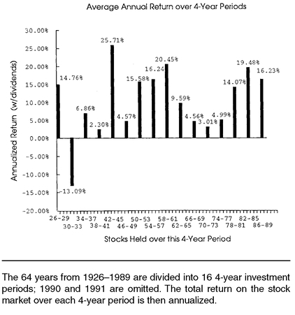
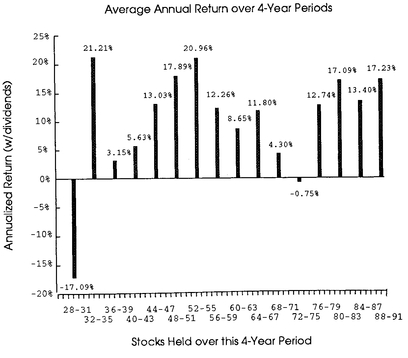
Figure 1-4a, where instead of looking at one-year investments, we look at four-year periods. Only the worst period (the Great Depression) shows a loss. The annualized return over longer time periods is less variable, because the randomness of the returns causes them to “average out.”
We could also look at the most recent 64 years, sliced into 4-year periods beginning in 1928. This similar analysis is shown in
Figure 1-4b; the results differ slightly. While still less variable than single-year returns, these 4-year returns show a different pattern with more losses.
Distribution of Market Returns
The risky nature of the stock market causes many people to mistakenly view it as a form of gambling. Yes, the outcome is uncertain and, as in a casino, you can lose your money. But in the stock market, the “house” doesn’t take a cut (although your broker or management company certainly will). On average, you will lose money in a casino; on average, you will win money or earn some positive return in the stock market (e.g., the +12% average noted above). In either case, the longer you “play,” the more certain these outcomes are. Also, unlike the potentially disappearing bankroll you take into the casino, there is no way the value of your diversified stock portfolio or fund will ever go to zero (even though any individual stock might).
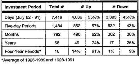
Let’s have a look at the historical data on market gains and losses—it is quite interesting and instructive. There were 792 months of market return data between 1926 and 1991; also, daily data were analyzed from the period July 1962 to December 1991. The results are tabulated in
Table 1-1. Almost 55% of the daily returns were positive—in a typical 22-day month, the market would have had 12 up days and 10 down days. For longer periods, note the increasing probability of a gain in the market over that period.
The market tends to rise over time. Over just a brief instant of “market time,” this trend is indiscernible. Over a full day, you can see the tendency, but the random “bounce” around the trend still causes a large number (45½%) of down periods. But as we allow more time, the upward trend compounds, while at the same time the random bounces average each other out. So as time increases, we are more assured of getting a positive return out of the market. This characteristic of the market explains the typical advice from investment advisors to put into the stock market only your “five-year-andout” funds. That is, if you might need access to your funds within the next five years or sooner, it may not all still be there (if invested in the stock market) due to risk of loss; but funds invested for longer periods are less likely to experience a loss.
TABLE 1-1 Counting the Stock Market’s Ups and Downs

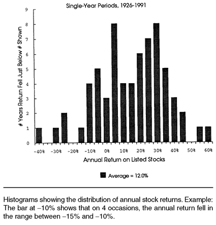
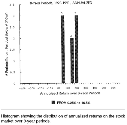
We can also look at the actual distribution of returns over various time periods to develop a better sense of the risk of the marketplace. A histogram, or bar chart, of annual returns is shown in
Figure 1-5, which has a different format from the previous ones; now the annual return is shown along the horizontal axis. The
number of times that a particular return occurs is on the vertical axis. The annual returns are grouped into ranges of five percentage points. Reading from left to right, we see that there was one year during which the return was below −40%, one year when it was between −35% and −30%, and two years when it fell by −30% to −25%. You can verify this by looking again at the time series of annual returns in
Figure 1-3 above. Note that even though the distribution is centered over the 12% average annual return, the actual return has fallen in the +10% to +15% range during only four years out of the 66 years in the sample. Thus, if one were to say “The expected return on the market is 12%,” this would not mean that we really
expect the return to be +12%. Instead, this statement of
expectation really means that
on aver age, we expect the random returns to vary around (or to center on) +12%. After the fact, of course, we can disparage any such predictions, but this does not mean there is no need for (or value in) making reasoned predictions at all. Pro football quarterbacks manage to keep their jobs despite the self-proclaimed superiority of thousands of Monday-morning quarterbacks.
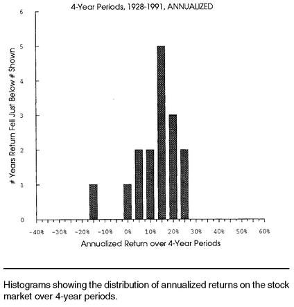
Figure 1-6 takes the stock returns from four-year periods (also shown year by year in
Figure 1-4b) and similarly displays the distribution of returns. Whereas the center (12%) of the distribution doesn’t change, the variability decreases. There are no prolonged huge gains or losses, as there were over the shorter single-year periods.
Figure 1-7 breaks the last 64 years into eight 8-year periods and displays the distribution of returns. Over this very long time period, the variability of returns was quite small, ranging from no gain to a 16.5% (annual average) gain. Over very long periods, we see neither serious losses nor extreme gains in the stock market.
Risk and Expected Return
Different types of investments will be “rewarded” with different expected returns. Both common sense and the historical data tell us this. We now examine the historical performance of a few basic types of investments and apply these lessons of the past to estimate what you can expect from your investments (on average) in the future.
Investments of increasing risk
3 have historically provided higher returns.
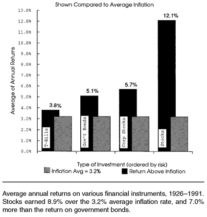
Figure 1-8 shows the average annual return over the 1926-1991 period for four broad classes of assets
4, and it displays them in relationship to the average 3.2% inflation rate for the period.

The shortest-term Treasury bills bear almost no price risk (variability), but have returned only 3.8% on average; that’s only about one-half percent over inflation. Longer-term Treasury bonds returned 5.1%, over a percentage point higher for taking the extra price risk. Bond prices can exhibit a lot of variation, as bond investors were surprised to find out over the past two decades. Corporate bonds are even riskier because they experience the same “duration-based” price risk that long-term Treasuries do, plus additional risk associated with default. The reward for these risks over time has not been great; top-grade corporates returned 5.7% over the period, or about one-half point more than Treasuries. The stock market has garnered far higher returns, which should not be surprising now that you are familiar with the high level of risk that had to be borne in the market. The 12.1% average return on stocks exceeds inflation by 8.9%, beats out T-bills by 8.3%, and surpasses the return on government bonds by 7.0%.

What about the future? Do the 66 years of returns analyzed portend a 12% expected annual return for the future? Not quite. First, there is no guarantee that the next 66 years will be anything like the past. Second, it is the relative return, not the absolute return, that gives us potentially useful information from past results. That is, if the basic risk differences between stocks and bonds persist into the future, then the basic return differences between them will probably continue as well. Higher returns will be demanded by investors to take the higher risk inherent in stocks, so, on average, stocks will have to give higher returns than bonds. The most relevant number to project into the future seems to be the 7% difference between common stock and government bond returns. With long-term government bond rates at 7-8% as of 1992, this would make the expected return on the stock market 14-15%. Although the assumptions that go into this projected return are reasonable, different sets of assumptions could result in very reasonable market return projections in the 12% to 16% range.
Now we can factor in the expected risk with this expected return to get a rough assessment of the probability of likely outcomes if you are invested in the stock market. Annual returns in the market had a standard deviation of 20.8% over the period analyzed. (See “Risk and Standard Deviation” in the box on page 17.)
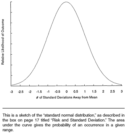
For a normal distribution, about two-thirds of repeated outcomes will fall into a range within one standard deviation of the average. That is, about two-thirds of the area under the relative likelihood curve would occur between −1 and +1 for the standard normal distribution as shown in
Figure 1-9.
For stock returns, about two-thirds of the years’ returns should fall into a range within one standard deviation of the average; for the past, this is roughly between −9% and +33%, using 12% as the center. Likewise, about 95% of the returns should fall into a range within two standard deviations on either side of the average.
So what’s likely to happen in future years in the stock market? Using the reasonable
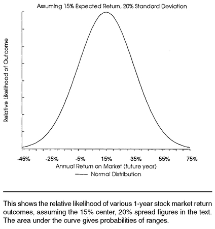
expectations of a 15% return and a 20% standard deviation around that expected return, we can make these reasoned guesses as to the probability of
future market outcomes (see
Figure 1-10):
• The return should be between −5% and +35% in roughly two out of three years.
• The return should be between −25% and +55% in all but one out of twenty years.
• You will make more than the 6% T-note rate about 67% of the time (two out of three years).
RISK and STANDARD DEVIATION
Whenever an outcome (such as next year’s return on the stock market) is random, it could take on many likely values. These outcomes or possible values have some expected value—also called the mean or average or center—around which they might “fall.” Suppose this average is 15%; that means that the possible outcomes, while random, will center on 15%. It would be nice to know how closely the possible returns occur near the average. If the spread of possible random returns is very large—say, if −50% and +60% returns were very likely—then we would say that the distribution of the random returns around their expected value (average) is very risky. The risk is that the actual outcome could end up very far (in either direction) from the expected value. In a less risky distribution, perhaps values outside the 0% to 30% range would be highly unlikely.
One way to measure this risk is called the standard deviation. This measure is, loosely, the typical distance (deviation) of the random value from their expected value (center). To be 1 standard deviation away from the average is not an unusual occurrence; to be 2 standard deviations away is unusual; to be 3 standard deviations away is quite rare. More exactly, the standard deviation is the square root of the variance; the variance is the average squared-distance from the expected value. A function (@std) in most spreadsheet packages will calculate the standard deviation of any range for you. The standard deviation is in the same units as the average—percent, in the case of stock returns.
Figure 1-9 is a sketch of the
standard normal distribution showing the relative likelihood of a random outcome compared to its expected value. Random outcomes are shown along the bottom scale, in terms of how far (how many standard deviations away) they are from the expected value or center. Note that it is most likely that random outcomes are near their expected value, and less and less likely to occur the further they are from their expected value. The probability that an outcome will fall in a particular range is given by the amount of the total area under the “bell-curve” that falls between those two numbers. For example, there is a 38.3% probability that the random value will fall between −0.5 and +0.5 standard deviations from the center. Other probabilities of falling within a certain distance of the expected value are:
68.3% within 1 s.d. ; 86.6% within 1.5 s.d.;
95.4% within 2 s.d.;
98.8% within 2.5 s.d. Only one-quarter of one percent of normal random values would be more than 3 standard deviations from the center.
Thus, a standard deviation is simply a measure of spread that allows us to “standardize” how far random values are spread about their center. This is useful for assessing the likelihood of various stock returns.
Figure 1-10 shows one possible random distribution of stock market returns, using the numbers in the text for center (15% expected return) and spread (20% standard deviation). The possible annual returns along the bottom of the sketch are marked in one standard deviation intervals (every 20%, centered around 15%). This allows us to make probability assessments of various returns, as presented in the text.
• You will have a positive return in about 77% of the years and lose money two years out of every nine.
• You will lose more than −10% about one year in ten.
• Your chances of losing money over a full four-year period of investment is only about 6%-7%.
• Over a ten-year period, the odds are 7-to-1 that your market return will average better than the current long-term government bond interest rate.
• The market will have a “big year” of a 25% or higher gain roughly every three years.
These numbers are nothing more than educated guesses backed up by reasonable assumptions and analyses. They are not meant to entice or scare you, only to give you some estimate of what you’re getting into. Note that these numbers apply to the returns (including dividends) on the market as a whole, and not to a particular stock, industry, or other undiversified investment. As the advertisements say, “Your mileage may vary!”
MARKET TIMING AND FORMULA STRATEGIES
Being able to time the market is certainly one of every investor’s dreams. Knowing when the market has peaked or how to distinguish a market correction from the seemingly identical start of a bear market is beyond the capabilities of mere mortals (except in retrospect, when many would-be market oracles claim to have accomplished this feat). But our failings are not from lack of trying. There are thousands of market professionals whose main purpose is to “call” turns in the market or to advise investors or clients when to switch between asset types.
Timing the Market
Despite the exhortations of many who study financial markets to assume a buy-and-hold posture in the market, the temptation to actively pursue timing strategies wins over many investors. A look back at the numbers may help you understand why. Using a buy-and-hold strategy, an investor with $100 at the end of 1925 would have accrued $53,364 by the end of 1991 (a 9.98% compound annual return). If this investor had been lucky enough to pull her money out of equity investments just prior to all “down” years and just keep it in a mattress, her 1991 fund would have been $981,848 instead (a 14.94% compound annual return). This would have involved 15 round-trip, end-of-year switches out of and into the stock market. If only 4 well-timed switches had been allowed, instead of 15, she still could have had $526,012 by 1991, a 13.86% compound annual return.
The problem with this is obvious—you just never know beforehand when to move your money into and out of the market. Individual investors, as motivated as they are to buy low and sell high, invariably have this incredible knack for doing just the opposite. It’s so easy to get wrapped up in the euphoria of a raging bull market and buy high, or be scared into selling low by the “sky is falling” bear market mentality, that most attempts by small investors to time the market are doomed to failure. Look at a poor investor who had the misfortune to “reverse-time” the market in the worst way over our 66-year market period. By moving into and out of the market at the end of the worst possible years, the $100 in 1925 could have dwindled to roughly the cost of a Big Mac and fries (with no drink) by 1991. I don’t personally know any of the extreme investors described above, but we all certainly know of “timers” who more frequently resemble this latter unfortunate case than the former. In fact, many market technicians and professionals tend to use levels of small investor sentiment such as odd-lot sales, mutual fund inflow/outflow statistics, and investor surveys to gauge when the market is overbought or saturated (indicators that are too positive supposedly portend a down market), or when investor depression is a potential precursor to a turn upward.
Automatic Timing with Formula Strategies
The rewards to successful timing are substantial, but individual investors, in particular, seldom reap them. Many investors have found that they need a disciplined approach to help them avoid the herd mentality that often leaves their ill-timed investments underperforming the market. This is where formula strategies enter the picture.
Whereas typical timing strategies involve active decisions about moving money into and out of the stock market (or other investments), formula strategies are nothing more than passive guidelines toward the same end. The idea is to proceed through the twisting, bumpy investment highway on cruise control, avoiding the excessive stop-and-go natural tendencies that seem to brake your investment vehicle in all the wrong places. Formula strategies are meant to be automatic and mechanical, the very antithesis of the emotional involvement inherent in timing strategies. Passive formula investing is not meant to beat the market but merely to survive in it and end up with the proper reward for the risk incurred. As we have seen, mere survival in the market grants fairly substantial rewards that grow even more substantial over time. In our greed to beat the market, we often miss that simple point.
Also remember that if timing systems were developed that could truly consistently beat the market, they would not be viable for very long. If we all jumped on the same bandwagon, we’d all get the same return—the average return. If you’re looking for a surefire way to beat the market, this book will not likely provide it. The formula strategies we’ll encounter will provide a few sensible alternative methods of adjusting your market exposure and accumulating market wealth over time. They will, we hope, give you the investment returns you deserve to compensate you for risk while guiding you away from the trap that snares so many investors—that of buying high, then panicking and selling low.
As mentioned earlier, the most popular formula strategy is dollar cost averaging, summarized in Chapter 2. Value averaging is a variation of dollar cost averaging that will be introduced in its simplest form in Chapter 3. Several variations of dollar cost averaging and value averaging will be presented and analyzed to help you tailor a strategy that suits your needs. The number of different formula strategies that could be devised is limited only by one’s imagination. You will find that no one strategy is strictly better than all the others, but that each has its own specific flavor that will appeal to different investors in different ways. By “paper-trading” many of these strategies against actual market data and simulated possible future markets, as is done in this book, you should be able to get a reasonable feel for the capabilities and limitations of these strategies. This should help you pick out one that is comfortable for you to use in accumulating your own wealth over time.
ENDNOTES
1 All historical market data used are calculated from CRSP daily and monthly value-weighted market index return series. This index takes all stocks listed on the NYSE and AMEX and constructs a weighted average based on each stock’s total market capitalization, thus giving an accurate indication of the total value of the combined stocks on both markets.
2 This 12% average does not contradict the 9.98% compounded growth rate quoted earlier. This higher 12% figure is obtained simply by averaging all of the various annual returns; the lower 9.98% figure is calculated by figuring out the
constant rate at which the beginning value would have to increase to grow to the final actual value. This is the difference between an
arithmetic mean and a
geometric mean. A simple example is a $100 stock that falls to $50 (−50%) one year, and then rebounds (+100%) back to $100 the second year. The arithmetic mean, or average, of the two (−50%, +100%) annual figures is +25%, but the compound annual growth rate to get from beginning ($100) to end ($100) was clearly + 0%. Arithmetic means are always higher than geometric means. This means that the
average of returns from several periods will always be a number higher than the actual
compound return per period.
3 The working definition of
risk as used here is the expected standard deviation (typical variation from the average) of annual returns. This is not exactly the right kind of risk to associate with the expected returns on individual assets—finance practitioners use measures of
market risk (such as
beta) for stocks that are more complex. But for the purposes used here (differentiating broad classes of assets), the more basic measure of risk works fine.
4 T-bill and stock data are from CRSP data set. Ibbotson and Sinquefield’s
Stocks, Bonds, Bills and Inflation reports similar numbers for the period ending in 1991. (Chicago: Ibbotson Associates, published annually.) Their numbers are used for bond returns.
2006 NOTE
The stock market has been through some exciting times since this book’s original publication. An updated look at the past 16 years (1990—2005) shows that our recent market history is surprisingly consistent with the long-term averages presented in Chapter 1.
Using the S&P 500 Index, or the more broad-based Russell 3000 or Wilshire 5000, the market’s 1990—2005 annual returns were much like those in the prior 64-year history—just a bit less volatile:
• +12% average return
• 17%-18% standard deviation
The 16 annual results were close to, but slightly under, the Chapter 1 statistical predictions:
• Four losing years, two of them worse than -10%
• One flat year
• Nine double-digit gains, five better than +25%
Looking
forward, though, most experts agree that the
expected return on the market now is lower than had been predicted in the early 1990s. This is, simplistically, due to today’s low level of interest rates and market volatility. In today’s 5% interest rate environment, the expected return on the broad stock market is likely 9 to 10%—much lower than the 14 to 15% described in Chapter 1. And instead of 20% volatility, today’s forward-looking estimate would be a standard deviation in the 13 to 16% range. Here are a few probability estimates based on these updated figures:
• Expect returns between -5% and +25% two years out of three.
• Look for returns between -20% and + 40% in all but one year in twenty.
• Expect the market to outperform the 5% interest rate 63% of the time (5 years in 8).
• Expect 75% positive returns; lose money one year in four.
• Look for a “big year” of over 20% gain roughly one year in four.
