8
Comparing the Strategies
This chapter looks at hundreds of simulated markets (as described in Chapter 7) to evaluate dollar cost averaging, value averaging, and several variations that have already been discussed. We have already accomplished this comparison in Chapters 2-6 using actual historical market data. The results you will see using market simulations should not surprise you too much. These results should, however, give you a much better feel for how the various strategies do under different circumstances that you have not seen or been able to evaluate with the historical data. This type of simulated comparison is useful in answering typical questions that interested readers tend to have.
FIVE-YEAR SIMULATION RESULTS
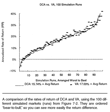
The first 100 simulated runs of our five-year random market (as shown in
Figure 7-2) were used to evaluate the dollar cost averaging and value averaging strategies in their “pure” or “fixed-amount” forms. The rates of return are displayed, ordered worst to best from left to right in
Figure 8-1. This is
not a time-series. You are
not looking at how an investment evolves over 100 consecutive periods; instead, each symbol represents the rate of return over a separate, complete 5-year simulated investment. For each simulation, the vertical position of the line shows the IRR (rate of return) for dollar cost averaging, and the symbol above or below the line shows the IRR with value averaging. The rate of return with value averaging exceeds that with dollar cost averaging (i.e., the symbol is above the line) on 84 out of 100 occasions. The average of all 100 rates of return from each strategy are shown in the legend of the figure: value averaging returned 17.03% on average, compared to 15.74% with dollar cost averaging, and 15.23% with the constant share strategy (not shown). The average returns were slightly more variable (riskier) with the DCA strategy.
1 The best relative performance of value averaging was a +6.05% higher return than DCA; the worst of the 16 losers was −3.09% lower than DCA. Over these 100 simulated 5-year markets, the final share price ended up lower than it started on six occasions (as was noted in
Figure 7-2). The CS strategy provided negative returns 7 times, dollar cost averaging was negative 6 times, and the value averaging strategy had negative returns only 3 times out of 100 simulations.
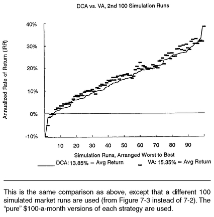
Figure 8-2 shows exactly the same exact comparison as in
Figure 8-1, except that the
second 100 runs of the random simulation, instead of the first 100 (as previously shown in
Figure 7-3) are used as the basis of comparison. This time, value averaging has returns that average 1.50 percentage points higher (15.35% over 13.85%) than dollar cost averaging, and it has higher returns 90 times out of the 100 simulations shown.
When this comparison of the pure strategies was repeated again and again using different runs of the simulation, the results were not terribly different.
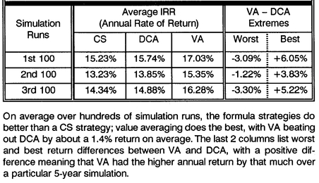
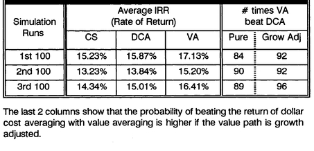
Table 8-1 shows the average results for the first three different 100-runs of the simulation.
First 3 Sets of 100 Runs of Simulation
The table further shows that value averaging tends to outperform dollar cost averaging by over a 1% higher return, whereas dollar cost averaging outperforms constant share purchases by about one-half point. Only rarely was the return difference between strategies in a given simulation extreme; the wildest (6.05% better for VA, 3.30% better for DCA) return differences are shown in the last 2 columns. Whereas value averaging outperformed dollar cost averaging in only 84 out of the first 100 runs, it was best on 90 and 89 occasions (respectively) over the next two sets of 100 runs of the simulation. You may recall from Chapter 3 that the relative comparison for historical data had a similar score, in that value averaging had “won” 52 of the last 62 overlapping 5-year investment periods. The simulation results show that you could expect slightly better than this historical result out of value averaging in the future.
Using Growth Adjustments
Having compared the strategies in their so-called pure forms, we now look at how they perform when adjusted for expected market growth (as recommended in Chapters 4 and 5).
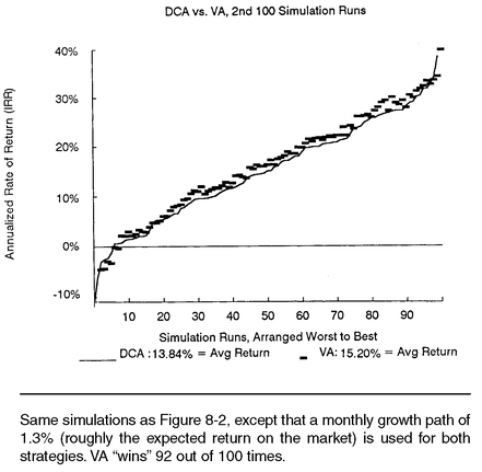
Figure 8-3 shows the performance of the strategies over the second 100 simulation runs, where each strategy used a growth factor of 1.3% per month.
2 Growth adjustments have little effect on the returns from dollar cost averaging; the effect on value averaging is mixed.
3 The number of times the value averaging strategy has the higher rate of return increases to 92 times out of 100. Due to the compounding increase (growth adjustment) of the value path, the variation of returns (the risk) increases slightly with a growth-adjusted value averaging strategy.
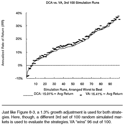
Figure 8-4 is exactly like
Figure 8-3, except that the performance of the strategies is evaluated over the
third 100 simulation runs, again using a growth factor of 1.3% per month.
Both strategies perform better (after growth adjustment) over this set of simulations; both increase in average absolute return by about 0.125%. Value averaging outperforms dollar cost averaging on 96 out of 100 runs, compared to only 87 runs using the same simulations but without any growth adjustments.
When this comparison of the growth-adjusted strategies was repeated again and again using different runs of the simulation, the results were not terribly different.
Table 8-2 shows the average results for the first three different 100-runs of the simulation.
Table 8-2 Comparison of “Growth-Adjusted” Strategies
First 3 Sets of 100 Runs of Simulation
There seem to be theoretical, performance, and commonsense reasons for applying some growth adjustment to whatever formula strategy you use. Higher rates of growth (in the amount you invest), which exceeded even the most optimistic expected market returns, were also analyzed. The numbers (not shown) weren’t terribly different from what you see in
Table 8-2, and there appears to be little return advantage to using extreme growth levels in planning your investment quantities. As you might suspect, both strategies are made riskier by the use of above-market growth factors, and value averaging is affected the most in that respect.
No-Sell Variation
Chapter 6 discussed the possibility of doing nothing when the value averaging strategy “dictates” selling shares, and analyzed that variation using actual market data.
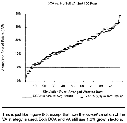
Figure 8-5 displays the results of
no-sell value averaging compared to dollar cost averaging in exactly the same scenario as in
Figure 8-3. Both strategies are growth-adjusted, and the second set of 100 simulations is used.
As suspected, failing to follow the sell recommendations of the value averaging strategy did have an adverse impact on performance—but not as much as you might suspect. In the simulation shown, the reduction in average annual return was only −0.14%; in the other two hundred simulations the reduction was −0.18% and −0.16%. By using the no-sell variant, you are only giving up about one-eighth of the return advantage of the value averaging strategy.
Volatility
By straying from the expected market parameters of center and spread discussed in the previous chapter, we can begin to understand how volatility affects the relative performance of the strategies. Because value averaging operates by taking advantage of large moves in either direction, you might suspect that the relative return advantage of value averaging will increase with volatility.
Some simulations are performed for markets with only half the typical volatility, and then with double volatility. If the standard deviation of monthly returns is reduced to 2.75% (half of the 5.5% figure used throughout this chapter), the average relative return advantage of value averaging diminishes significantly (but is still positive). When the volatility is 11%, or double the normal figure, the return difference between strategies increases substantially. The average rate of return advantage of a pure value averaging strategy over 100 simulation runs in these situations is:
• +0.38% with half the volatility;
• +1.50% with standard volatility; and
• +5.76% with double volatility.
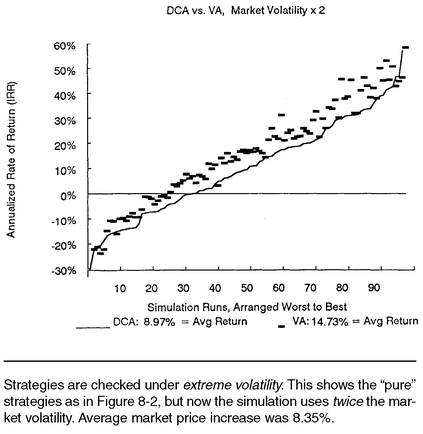
Results of the double volatility simulation are presented in
Figure 8-6. In this simulation, the pure value averaging strategy averaged an annualized return of 14.73%, compared with the return of 8.97% with dollar cost averaging, and only 6.62% for constant share purchases (not shown). The largest return advantage out of the 100 runs was a +15.67% difference between value averaging and dollar cost averaging; the worst performance was a −2.86% decrease in return due to value averaging. In 94 of the 100 simulations, value averaging came out on top. When this experiment was repeated again with another 100 different simulation runs, there was a 5.83% average return advantage for value averaging, which “won” on 97 out of 100 runs. Changing the strategies by adjusting for growth and by not selling did not make the results any better for value averaging than what we have just seen.
All the strategies obviously became riskier when volatility increases. Interestingly, although the relative risk of value averaging does increase (over DCA) a bit with volatility, it is not a very significant increase. Still, the fact is that value averaging results in less investment exposure and value than dollar cost averaging portfolios when prices go way up, and in more investment exposure when prices go way down. Thus, it is still important to pick out a diversified investment vehicle (to avoid bankruptcy risk) with which to implement value averaging or any other contrarian
4 formula strategy.
TWENTY-YEAR SIMULATION RESULTS
Absolute or total market volatility increases over time,
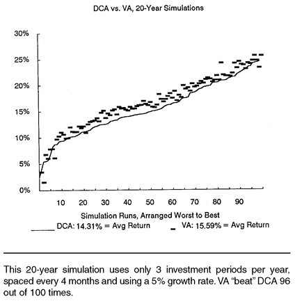
5 so you might suspect that the relative return advantage of value averaging would increase substantially over time. It does not seem to. A 20-year simulated market was constructed, and investments were made at 4-month intervals using the standard annual market return parameters. A growth adjustment of 5% per period (about 15% per year) was applied to both strategies. The results are represented in
Figure 8-7.
Over 100 runs of the simulated market, the value averaging strategy outperformed dollar cost averaging 96 times. The compound average annual return for value averaging was 15.59%, comparing favorably with 14.31% for dollar cost averaging, and 13.66% for constant share purchases (not shown). The relative effectiveness of value averaging is related to the volatility per unit time.
SUMMARY
We’ve just “paper-traded” several variations of the investment strategies to see how they would perform under a wide range of plausible market conditions. Under these simulations, in most cases value averaging performs better than the other strategies and gives higher returns on average. The market simulation was a true “random walk,” so conceivably these results could be expected in real markets. This is really true only if stock market returns are truly random. This point will be discussed at length in Chapter 9.
ENDNOTES
1 The variation of the returns gives you some sense of the risk involved in the strategies. The standard deviation of the 100 annualized 5-year returns was 11.16% for dollar cost averaging and 10.73% for value averaging. Although value averaging was the less-risky strategy here, it was about equivalent in risk to dollar cost averaging on average, over the total of thousands of simulations done on different variations using different runs of market prices.
2 The dollar cost averaging strategy used a growing monthly investment amount, increasing the original $100 investment at 1.3% per month. Value averaging used a 1.3% growth factor as described in Chapter 5. The value path for month
t was:
Vt= 100 × t × (1 + 0.013)t
Thus, the value path started at $100 and grew to $13,023 over the 5-year period.
3 In this case, the average effect of growth adjusting is to decrease the average relative advantage and absolute return on value averaging (from 15.35% to 15.20%). Over more simulations, growth adjusting (on average) tends to increase the absolute return on value averaging, with no effect or perhaps an insignificant decrease in the
relative return advantage on value averaging over dollar cost averaging.
4 Contrarian strategies invest in something that is out of favor. Formula strategies such as value averaging are contrarian across time, investing the most in the market when it is in the least favor (prices are low), cutting against the popular investment trend.
5 It is much more likely that the price of a $100 stock is outside a range of $80-$120 after a decade than after a month. This “total volatility” is a different concept than “annualized” or average volatility, which decreases over time (as you saw in previous chapters). As time increases,
total volatility increases by the square root of time, but
average volatility per period
decreases by the square root of time. A simplified example: If the standard deviation of return over
1 year is 20%, what happens over a
4-year period? The square root of the time increase (four) is two. So
total volatility over the entire 4-year period doubles to 40%; thus,
average volatility each year is halved to 10% per year.
