
It is important to classify algorithms based whether they solve a given computational problem and, if so, how quickly. Similarly, it is important to classify computational problems based whether they can be solved and, if so, how quickly.
Estimate Duration: To estimate how long an algorithm or program will run.
Estimate Input Size: To estimate the largest input that can reasonably be given to the program.
Compare Algorithms: To compare the efficiency of different algorithms for solving the same problem.
Parts of Code: To help you focus your attention on the parts of the code that are executed the largest number of times. This is the code you need to improve to reduce the running time.
Choose Algorithm: To choose an algorithm for an application:
Time and Space Complexities Are Functions, T(n) and S(n): The time complexity of an algorithm is not a single number, but is a function indicating how the running time depends on the size of the input. We often denote this by T(n), giving the number of operations executed on the worst case input instance of size n. An example would be T(n) = 3n2 + 7n + 23. Similarly, S(n) gives the size of the rewritable memory the algorithm requires.
Ignoring Details, Θ(T(n)) and O(T(n)): Generally, we ignore the low-order terms in the function T(n) and the multiplicative constant in front. We also ignore the function for small values of n and focus on the asymptotic behavior as n becomes very large. Some of the reasons are the following.
Model-Dependent: The multiplicative constant in front of the time depends on how fast the computer is and on the precise definition of “size” and “operation.”
Too Much Work: Counting every operation that the algorithm executes in precise detail is more work than it is worth.
Not Significant: It is much more significant whether the time complexity is T(n) = n2 or T(n) = n3 than whether it is T(n) = n2 or T(n) = 3n2.
Only Large n Matter: One might say that we only consider large input instances in our analysis, because the running time of an algorithm only becomes an issue when the input is large. However, the running time of some algorithms on small input instances is quite critical. In fact, the size n of a realistic input instance depends both on the problem and on the application. The choice was made to consider only large n in order to provide a clean and consistent mathematical definition.
See Chapter 25 on the Theta and BigOh notations.
Definition of Size: The formal definition of the size of an instance is the number of binary digits (bits) required to encode it. More practically, the size could be considered to be the number of digits or characters required to encode it. Intuitively, the size of an instance could be defined to be the area of paper needed to write down the instance, or the number of seconds it takes to communicate the instance along a narrow channel. These definitions are all within a multiplicative constant of each other.
An Integer: Suppose that the input is the value N = 8,398,346,386,236,876. The number of bits required to encode it is Size(N) = log2(N) = log2(8,398,346,386,236,876) = 53, and the number of decimal digits is Size(N) = log10(8,398,346,386,236,876) = 16. Chapter 24 explains why these are within a multiplicative constant of each other. The one definition that you must not use is the value of the integer, Size(N) = N = 8,398,346,386,236,876, because it is exponentially different than Size(N) = log2(N) = 53.
A Tuple: Suppose that the input is the tuple of b integers I =  x1, x2, …, xb
 . The number of bits required to encode it is Size(I) = log2(x1) + log2(x2) + · · · + log2(xb) ≈ log2(xi) · b. A natural definition of the size of this tuple is the number of integers in it, Size(I) = b. With this definition, it is a much stronger statement to say that an algorithm requires only Time(b) integer operations independent of how big the integers are.
A Graph: Suppose that the input is the graph G = V, E with |V| nodes and |E| edges. The number of bits required to encode it is Size(G) = 2 Size(node) · |E| = 2 log2(|V|) · |E|. Another reasonable definition of the size of G is the number of edges, G(n) = |E|. Often the time is given as a function of both |V| and |E|. This is within a log factor of the other definitions, which for most applications is fine.
Definition of an Operation: The definition of an operation can be any reasonable operation on two bits, characters, nodes, or integers, depending on whether time is measured in bits, characters, nodes, or integers. An operation could also be defined to be any reasonable line of code or the number of seconds that the computation takes on your favorite computer.
Which Input: T(n) is the number of operations required to execute the given algorithm on an input of size n. However, there are 2n input instances with n bits. Here are three possibilities:
A Typical Input: The problem with considering a typical input instance this is that different applications will have very different typical inputs.
Average or Expected Case: The problem with taking the average over all input instances of size n is that it assumes that all instances are equally likely to occur.
Worst Case: The usual measure is to consider the instance of size n on which the given algorithm is the slowest, namely, T(n) = maxI∈{I | | I|=n} Time(I). This measure provides a nice clean mathematical definition and is the easiest to analyze. The only problem is that sometimes the algorithm does much better than the worst case, because the worst case is not a reasonable input. One such algorithm is quick sort (see Section 9.1).
Time Complexity of a Problem: The time complexity of a problem is the running time of the fastest algorithm that solves the problem.
EXAMPLE 23.1 Polynomial Time vs Exponential Time
Suppose program P1 requires T1(n) = n4 operations and P2 requires T2(n) = 2n. Suppose that your machine executes 106 operations per second. If n = 1,000, what is the running time of these programs?
Answer:
1. T1(n) = (1,000)4 = 1012 operations, requiring 106 seconds, or 11.6 days.
2.  operations. The number of years is
 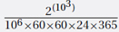 . This is too big for my calculator. The log of this number is 103 × log10(2) − log10106 − log10(60 × 60 × 24 × 365) = 301.03 − 6 − 7.50 = 287.53. Therefore, the number of years is 10287.53 = 3.40 × 10287. Don’t wait for it.
EXAMPLE 23.2 Instance Size N vs Instance Value N
Two simple algorithms, summation and factoring.
The Problems and Algorithms:
Summation: The task is to sum the N entries of an array, that is, A(1) + A(2) + A(3) + · · · + A(N).
Factoring: The task is to find divisors of an integer N. For example, on input N = 5917 we output that N = 97 × 61. (This problem is central to cryptography.) The algorithm checks whether N is divisible by 2, by 3, by 4, … by N.
Time: Both algorithms require T = N operations (additions or divisions).
How Hard? The summation algorithm is considered to be very fast, while the factoring algorithm is considered to be very time-consuming. However, both algorithms take T = N time to complete. The time complexity of these algorithms will explain why.
Typical Values of N: In practice, the N for factoring is much larger than that for summation. Even if you sum all the entries on the entire 8-G byte hard drive, then N is still only N ≈ 1010. On the other hand, the military wants to factor integers N ≈ 10100. However, the measure of complexity of an algorithm should not be based on how it happens to be used in practice.
Size of the Input: The input for summation contains is n ≈ 32N bits. The input for factoring contains is n = log2 N bits. Therefore, with a few hundred bits you can write down a difficult factoring instance that is seemingly impossible to solve.
Time Complexity: The running time of summation is 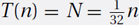 , which is linear in its input size. The running time of factoring is T(N) = N = 2n, which is exponential in its input size. This is why the summation algorithm is considered to be feasible, while the factoring algorithm is considered to be infeasible.
EXERCISE 23.1.1 (See solution in Part Five.) For each of the two programs considered in Example 23.1, if you want it to complete in 24 hours, how big can your input be?
EXERCISE 23.1.2 In Example 23.1, for which input size, approximately, do the programs have the same running times?
EXERCISE 23.1.3 This problem compares the running times of the following two algorithms for multiplying:
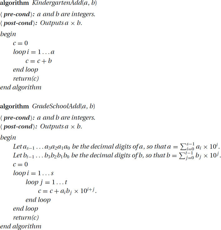
For each of these algorithms, answer the following questions.
1. Suppose that each addition to c requires time 10 seconds and every other operation (for example, multiplying two single digits such as 9 × 8 and shifting by zero) is free. What is the running time of each of these algorithms, either as a function of a and b or as a function of s and t? Give everything for this entire question exactly, i.e., not BigOh.
2. Let a = 9,168,391 and b = 502. (Without handing it in, trace the algorithm.) With 10 seconds per addition, how much time (seconds, minutes, etc.) does the computation require?
3. The formal size of an input instance is the number n of bits needed to write it down. What is n as a function of our instance a, b?
4. Suppose your job is to choose the worst case instance a, b (i.e., the one that maximizes the running time), but you are limited in that you can only use n bits to represent your instance. Do you set a big and b small, a small and b big, or a and b the same size? Give the worst case a and b, or s and t, as a function of n.
5. The running time of an algorithm is formally defined to be a function T(n) from n to the time required for the computation on the worst case instance of size n. Give T(n) for each of these algorithms. Is this polynomial time?
>EXERCISE 23.1.4 (See solution in Part Five.) Suppose that someone has developed an algorithm to solve a certain problem, which runs in time T(n, k) ∈ Θ(f(n, k)), where n is the size of the input, and k is a parameter we are free to choose (we can choose it to depend on n). In each case determine the value of the parameter k(n) to achieve the (asymptotically) best running time. Justify your answer. I recommend not trying much fancy math. Think of n as being some big fixed number. Try some value of k, say k = 1, k = na, or k = 2an for some constant a. Then note whether increasing or decreasing k increases or decreases f. Recall that “asymptotically” means that we only need the minimum to within a multiplicative constant.
1. You might want to first prove that g + h = Θ(max(g, h)).
2. 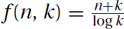 . This is needed for the radix–counting sort in Section 5.4.
3. 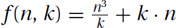 .
.
4. 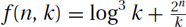 .
.
5. 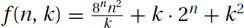 .
.
The Formal Definition of the Time Complexity of a Problem: As said, the time complexity of a problem is the running time of the fastest algorithm that solves the problem. We will now define this more carefully, using the existential and universal quantifiers that were defined in Chapter 22.
The Time Complexity of a Problem: The time complexity of a computational problem P is the minimum time needed by an algorithm to solve it.
Upper Bound: Problem P is said to be computable in time Tupper(n) if there is an algorithm A that outputs the correct answer, namely A(I) = P(I), within the bounded time, namely Time(A, I) ≤ Tupper(|I|), on every input instance I. The formal statement is

Tupper(n) is said to be only an upper bound on the complexity of the problem P, because there may be another algorithm that runs faster. For example, P = Sorting is computable in Tupper(n) = O(n2) time. It is also computable in Tupper(n) = O(n log n).
Lower Bound of a Problem: A lower bound on the time needed to solve a problem states that no matter how smart you are, you cannot solve the problem faster than the stated time Tlower(n), because such algorithm simply does not exist. There may be algorithms that give the correct answer or run sufficiently quickly on some input instances. But for every algorithm, there is at least one instance I for which either the algorithm gives the wrong answer, i.e., A(I) ≠ P(I), or it takes too much time, i.e., Time(A, I) ≥ Tlower(|I|). The formal statement is the negation (except for ≥ vs >) of that for the upper bound:

For example, it should be clear that no algorithm can sort n values in only  time, because in that much time the algorithm could not even look at all the values.
Proofs Using the Prover–Adversary Game: Recall the technique described in Chapter 22 for proving statements with existential and universal quantifiers.
Upper Bound: We can use the prover–adversary game to prove the upper bound statement ∃A, ∀I, [A(I) = P(I) and Time(A, I) ≤ Tupper(|I|)] as follows: You, the prover, provide the algorithm A. Then the adversary provides an input I. Then you must prove that your A on input I gives the correct output in the allotted time. Note this is what we have been doing throughout the book: providing algorithms and proving that they work.
Lower Bound: A proof of the lower bound ∀A, ∃I, [A(I) ≠ P(I) or Time (A, I) ≥ Tlower(|I|)] consists of a strategy that, when given an algorithm A by an adversary, you, the prover, study his algorithm and provide an input I. Then you prove either that his A on input I gives the wrong output or that it runs in more than the allotted time.
>EXERCISE 23.2.1 (See solution in Part Five.) Let Works(P, A, I) to true if algorithm A halts and correctly solves problem P on input instance I. Let P = Halting be the halting problem that takes a Java program I as input and tells you whether or not it halts on the empty string. Let P = Sorting be the sorting problem that takes a list of numbers I as input and sorts them. For each part, explain the meaning of what you are doing and why you don’t do it another way.
1. Recall that a problem is computable if and only if there is an algorithm that halts and returns the correct solution on every valid input. Express in first-order logic that Sorting is computable.
2. Express in first-order logic that Halting is not computable.
3. Express in first-order logic that there are uncomputable problems.
4. Explain what the following means (not simply by saying the same in words), and either prove or disprove it: ∀I, ∃A, Works(Halting, A, I).
5. Explain what the following means, and either prove or disprove it: ∀A, ∃P, ∀I, Works(P, A, I). (Hint: An algorithm A on an input I can either halt and give the correct answer, halt and give the wrong answer, or run forever.)