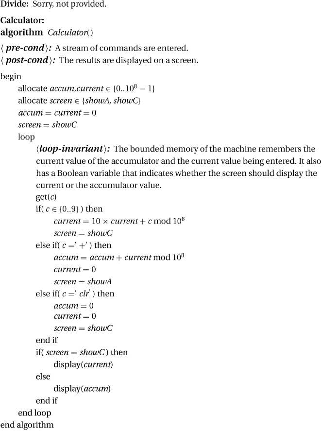
 .
.1.4.1 Selection Sort: If the input for selection sort is presented as an array of values, then sorting can happen in place. The first k entries of the array store the sorted sublist, while the remaining entries store the set of values that are on the side. Finding the smallest value from A[k + 1] … A[n] simply involves scanning the list for it. Once it is found, moving it to the end of the sorted list involves only swapping it with the value at A[k + 1]. The fact that the value A[k + 1] is moved to an arbitrary place in the right-hand side of the array is not a problem, because these values are considered to be an unsorted set anyway. The running time is computed as follows. We must select n times. Selecting from a sublist of size i takes Θ(i) time. Hence, the total time is Θ(n + (n−1) + · · · + 2 + 1) = Θ(n2) (see Chapter 26).
1.4.2 Insertion Sort: There are two steps involved in inserting an element into a sorted list. The most obvious step is to locate where it belongs. The second step to shift all the elements that are bigger than the new element one to the right to make room for it. You can find the location for the new element quickly using a binary search. However, it is easier to search and shift the larger elements simultaneously.
Linked List: Having the sorted elements stored in a linked list allows one to insert the new element in constant time. However, it then takes Θ(k) time to find where the new element goes.
Running Time: We must insert n times. Inserting into a sublist of size i takes Θ(i) time. Hence, the total time is Θ(1 + 2 + 3 + · · · + n) = Θ(n2).
Heap Sort: We will see in Section 10.4 that each of these steps can be done in Θ(log n) time when the elements are stored in a data structure called a heap.
1.4.3 The algorithm repeatedly passes through the array, swapping adjacent pairs if needed. After k such passes, the largest k elements have bubbled up to where they belong. Hence, it requires at most n passes until all elements are in place. Each pass requires n comparisons.
1.5.1 There are a number of problems.
1. A loop invariant shall to be a picture of the current state and not say what the iteration does. The loop invariant should simply be .
2. The loop invariant is not established correctly. With i = 1, the loop invariant requires  , not s = 0. The choice s = 0 and i = 0 would be better.
3. The loop invariant is not maintained correctly. Let s′ and i′ be the values of s and i when at the top of the loop. Let s″ and i″ be the values after going around again. The loop invariant gives that  . The code gives that s″ = s′ + i′ and i″ = i′ + 1. Together these give that
  . This is not
  as required, because i′ is being added in twice. i′ + 1 should be added in order to maintain the loop invariant.
4. The exit condition is not very well stated. An equivalent and easier-to-see exit condition would be “exit when i > I.”
5. The exit condition, i > I, and the loop invariant,  , together do not give the postcondition. Instead, they give that
  is returned.
6. The algorithm as a whole happens to work. A quick fix is to change the loop invariant to  .
.
Longest Block of Ones:

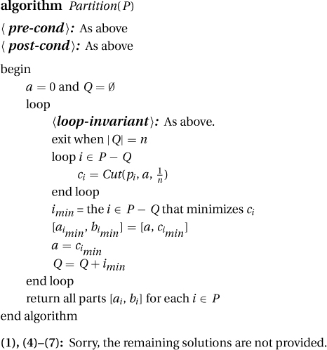
(2): The loop invariant is:
a. The beginning [0, a] of the cake has been partitioned into |Q| disjoint pieces.
b. Each player pi ∈ Q has been allocated a piece [ai, bi] worth at least  to him.
c. The remaining [a, 1] interval of the cake is worth at least (n − |Q|)/n to each of the remaining players, i.e., to those in P − Q.
(3):
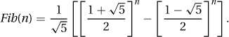
3.1.5 Instead of bounding the height given the number of nodes, it is easier to compute the reverse relation. Let N(h) be the minimal number of nodes in an AVL tree of height h. In order for a tree to be of height h, it must have at least one subtree of height h − 1. In order for it to be an AVL tree, the other subtree can differ by at most one, so it must have height at least h − 2. It follows that the number of nodes in this tree is at least N(h) = N(h−1) + N(h−2) + 1. Except for the +1 of the root, this is that same as the famous Fibonacci numbers defined by Fib(n) = Fib(n−1) + Fib(n−2). Exercise 27.2.1 goes on to prove that Fib(n) = Θ(αn), where  . If N(h) = Θ(αn), then H(n) = Θ(log n).
3.2.4 The tests will be executed in the order that they are listed. If next = nil is tested first and passes, then because there is an OR between the conditions, there is no need to test the second. However, if next.info ≥ key is the first test and next is nil, then using next.info to retrieve the information in the node pointed to by next will cause a run-time error.
4.4.1 Doing binary search in O(log(n × m)) time is impossible. See the lower bound in question (Exercise 7.0.7). If you take O(n log m) time doing binary search in each row, then you are taking too much time. It can be done by examining n + m − 1 entries. Observe that the values in the matrix increase from A[1, 1] to A[n, m]. Hence, the boundary between values that are less than or equal to x and those that are greater follows some monotonic path from A[1, m] to A[n, 1]. The algorithm traces this path starting at A[1, m]. When it is at the point A[i, j], the loop invariant is that we have stored the best answer from those outside the subrectangle A[i..n, 1..j]. Initially, this is true for [i, j] = [1, m], because none of the matrix is excluded. Now suppose it is true for an arbitrary [i, j]. The algorithm then compares A[i, j] with x. If it is better than our current best answer, then our current best is replaced. If A[i, j] ≤ x, then because the values in the row A[i, 1..j] are all smaller than or equal to A[i, j], these are worse answers, and hence we can conclude that we now have the best answer from those outside the subrectangle A[i + 1..n, 1..j]. We maintain the loop invariant by increasing i by one. On the other hand, if A[i, j] > x, then it is too big and so are all the elements in the column A[i..n, j] which are even bigger. We can conclude that we have the best answer from those outside of the subrectangle A[i..n, 1..j − 1]. We maintain the loop invariant by decreasing j by one. The exit condition is |i..n| = 0 or |1..j| = 0 (i.e., i > n or j < 1. When this occurs, the subrectangle A[i..n, 1..j] is empty. Hence, our best answer, which by the loop invariant is the best from those outside this subrectangle, must be the best overall. The measure of progress, |i..n| + |1..j| − 1 = (n − i + 1) + (j) − 1, is initially n + m − 1 and decrease by one each iteration. After n + m − 1 iterations, either the algorithm has already halted or the measure has reached zero, at which point the exit condition is definitely met.
(2): The loop invariant ℓ × r + s = x × y is established trivially by setting ℓ = x, r = y, and s = 0. Let ℓ′, r′, s′ be the values when at the top of the loop, and assume that ℓ′ × r′ + s′ = x × y.
In the first step, if ℓ′ is odd, then ℓ″ = ℓ′ − 1 and s″ = s′ + r′. This gives that ℓ″ × r″ + s″ = (ℓ′ − 1) × r′ + (s′ + r′) = ℓ′ × r′ + s′, which by the loop invariant is x × y.
In the second step, ℓ′′′ = ℓ″/2 and r′′′ = 2r″. This gives that ℓ′′′ × r′′′ + s′′′ = (ℓ″/2) × (2r″) + s″ = ℓ″ × r″ + s″, which by the loop invariant is x × y.
(4): The Ethiopians exit when ℓ = 1. But this being odd, they must add r to s. We will iterate one more time and exit when ℓ = 0. This exit condition gives s = ℓ × r + s, and the loop invariant gives ℓ × r + s = x × y. Hence, in the end s = x × y.
(1), (3), (5), and (6): Sorry, not provided.
7.0.2 The bound is n ≤ rt.
Each round, he selects one row; hence, there are r possible answers. After t rounds, there are rt possible combinations of answers.
The only information that you know is which of these combinations he gave you. Which card you produce depends deterministically (no magic) on the combination of answers given to you. Hence, depending on his answers, there are at most rt cards that you might output.
However, there are n cards, any of which may be the selected card. In conclusion, n ≤ rt.
The book has n = 21, r = 3, and t = 2. Because 21 = n ≤ rt = 32 = 9, the trick in the book does not work.
Two rounds is not enough. There need to be three rounds.
7.0.3 It is a trick question, because with a balance there are three, not two, outcomes and hence only log3 n operations are needed. Divide the objects into three piles, two of equal size and the third as close as possible. Put the first two piles on the scale. If one is heavier, then it contains the heavier object; otherwise the third pile does. Recurse on this one pile.
7.0.6 In the lower bound for parity, any starting input I would have worked equally well. Here, however, there is only one input that will work, and that is I being the all-zero string. This ensures that, as before, changing the jth bit of I, for any j ∈ J = [1, n], changes the answer from the AND being zero to the AND being one. This proves that any algorithm solving the problem requires time of at least n.
8.5.2 Ra: One might complain that if my instance is 〈n, m〉, then my friend’s instance cannot be 〈n − 1, 2m〉, because 2m is not smaller then m. However, we can define the size of instance 〈n, m〉 to be simply n. According to this measure, my friend’s instance is indeed smaller. Moreover, when the instance becomes of size zero or smaller, then n ≤ 0 and the recursion stops. We prove that the depth of recursion is at most n as follows. On instance 〈n, m〉, the size starts at n and decreases by at least one every level of recursion, so after n levels the size is at most zero and the algorithm stops recursing further. For example, starting with 〈5, 2〉, it recurses on 〈4, 4〉, 〈3, 8〉, … , 〈0, 64〉, and then halts.
Rb: One might claim that all is well because both friends get instances (〈n − 1, m〉 and 〈n, m − 1〉) that are smaller. However, for this to be true for both friends, the size must be something like n + m. However, according to this definition, the instance 〈5, −5〉 is small, but the algorithm does not halt. There is a path down this recursive tree that is infinite, namely 〈n, m〉, 〈n, m − 1〉, 〈n, m − 2〉, … 〈n, 1〉, 〈n, 0〉, 〈n, −1〉, 〈n, −2〉 … .
Rc: Here the size of the instance 〈n, m〉 can be defined to be n + m. According to this measure, each friend is given a smaller instance. Moreover, if the size on the instance is zero, then either n ≤ 0 or m ≤ 0. Either way the program halts. The depth of recursion can be at most n + m because this is the initial size and the size decreases by one each iteration.
Rd: Let the size of the instance 〈n, m〉 be 5n + 2m. Then the first friend’s instance 〈n − 1, m + 2〉 has size 5(n − 1) + 2(m + 2) = 5n + 2m − 1, which is one smaller. The second friend’s instance 〈n + 1, m − 3〉 has size 5(n + 1) + 2(m − 3) = 5n + 2m − 1, which is also one smaller. Moreover, if the size on the instance is zero, then either n ≤ 0 or m ≤ 0. Either way the program halts. The depth of recursion can be at most 5n + 2m because this is the initial size and the size decreases by one each iteration.
Re: I claim that there is a path down this recursion tree that is infinite. If my instance is 〈n, m〉, then my first friend has 〈n − 4, m + 2〉, his first friend has 〈n − 8, m + 4〉, his first friend has 〈n − 12, m + 6〉, his second friend has 〈n − 6, m + 3〉, and his second friend has 〈n, m〉 which is the same as my instance. This can be repeated infinitely often.
It is interesting that the last two examples can be generalized to the friend’s instances of size 〈n − a, m + b〉 and 〈n + c, m − d〉. If ad > bc then the program halts, else it does not.
Fun(1) = X
Fun(2) = Y
Fun(3) = AYBXC
Fun(4) = A AYBXC B Y C
Fun(5) = A AAYBXCBYC B AYBX C
Fun(6) = A AAAYBXCBYCBAYBXC B AAYBXCBYC C
8.7.2 To prove S(0), let n = 0 in the inductive step. There are no values k where 0 ≤ k < n. Hence, no assumptions are being made. Hence, your proof proves S(0) on its own.
9.1.1 Insertion sort and selection sort.
9.1.2 1. Given 〈a1, a2, … , an〉, I remove the last character an. I give 〈a1, a2, … , an−1〉 to my friend, and he returns the reversed tuple 〈an−1, … , a1〉 to me. I add an to the front of the tuple, producing 〈an, an−1, … , a1〉 as required. If my initial tuple has only zero (or one) element, then there is nothing to do.
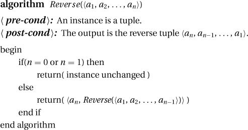
2. The iterative program has two (nonnested) loops. The first pushes each element on the stack, one at a time, starting with an. The loop invariant is that after i iterations what remains in the tuple is 〈a1, a2, …, an−i−1, an−i〉 and the stack contains 〈an−i+1, an−i+2, … , an〉 with an−i+1 at the top. At the i = 0 iteration, the loop invariant is trivially true. The next iteration removes the last element an−i from the tuple and pushes it on the stack. This maintains the loop invariant while making progress. In the end, with i = n, 〈a1, a2, …, an〉 is on the stack with a1 at the top. The second loop pops each element off the stack and puts it at the beginning of the tuple. The loop invariant is that after i iterations, the stack again contains 〈ai+1, ai+2, … , an〉 with ai+1 at the top, but now the tuple is 〈ai, ai−1, … , a2, a1〉. With i = n, the stack is empty and the tuple is 〈an, an−1, … , a2, a1〉.
3. Recursion is implemented on a computer, using a stack of stack frames. The first stack frame is given 〈a1, a2, … , an〉, and it removes and remembers the last character an. Its friend is the second stack frame, which is given 〈a1, a2, … , an−1〉. It removes and remembers its last character an−1. As we recurse deeper, the stack frames that have not yet completed are pushed on a stack. After i such stack frames, the loop invariant is that the the friend’s friend’s friend’s … friend is given the tuple 〈a1, a2, … , an−i−1, an−i〉 and the stack contains stack frames, each remembering one of the elements an−i+1, an−i+2, … , an, with an−i+1 at the top. Note this is the same loop invariant as the iterative program. The recursive base case is reached when i = n and the stack frame is given the empty tuple. Then, one at a time, in reverse order the stack frames complete their computations by each adding its element to the beginning of the tuple. The loop invariant is that after i such returns, the stack of stack frames is remembering ai+1, ai+2, … , an with ai+1 at the top, and the current stack frame is returning the tuple 〈ai, ai−1, … , a2, a1〉. Again, note that this is the same loop invariant as the iterative algorithm. With i = n, the stack is empty and the first stack frame returns the tuple 〈an, an−1, … , a2, a1〉.
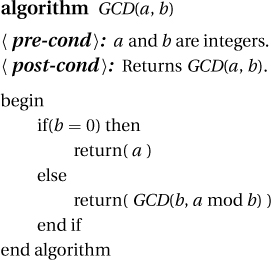
1). Given the integers a and b, the iterative algorithm creates two numbers x = b and y = a mod b. It notes that GCD(a, b) = GCD(x, y), and hence it can return GCD(x, y) instead of GCD(a, b). This algorithm is even easier when you have a friend. We simply give the subinstance 〈x, y〉 to the friend, and he computes GCD(x, y) for us. For the iterative algorithm, we need to make sure we are making progress, and for the recursive algorithm, we need to make sure that we give the friend a smaller instance. Either way, we make sure that in some way 〈x, y〉 is smaller than 〈a, b〉. For the iterative algorithm, we need an exit condition that we are sure to eventually meet, and for the recursive algorithm, we need base cases such that every possible instance is handled. Either way, we consider the case when y or b is zero. The resulting code is
2). We will need to understand this relationship y = a mod b better. Here y is the remainder when you divide a by b. If we let  , then a = r · b + y or y = a − r · b.
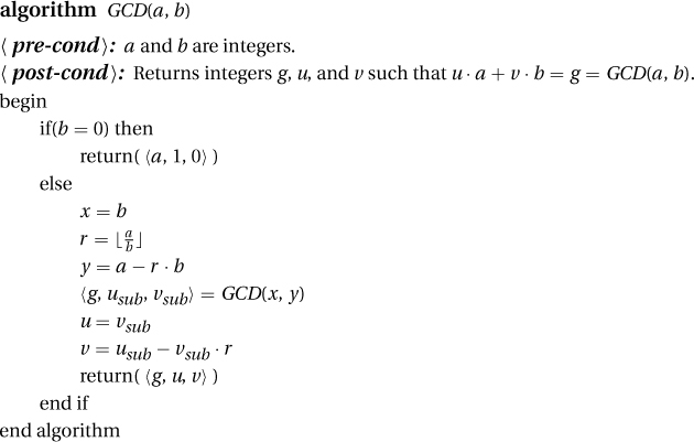
When we generalize the problem, the friend, in addition to g, also gives us usub and vsub such that usub · x + vsub · y = g = GCD(x, y) = GCD(a, b). Plugging in x = b and y = a − r · b gives usub · b + vsub · (a − r · b) = g, or vsub · a + (usub − vsub · r) · b = g. Hence, if we set u = vsub and v = usub − vsub · r, then we get u · a + v · b = g = GCD (a, b) as required. I simply provide these answers. For the base case with b = 0, we have g = GCD(a, b) = a. Hence, u = 1 and v = 0 gives that u · a + v · b = g = GCD(a, b). The resulting code is
3). Our goal is to find two integers U and V such that U · a + V · t = w. Then you give the storekeeper U of the a coins and V of the b coins for a total worth of w dollars. If U or V is negative, this amounts to the storekeeper giving you coins as change.
To find U and V, let’s start by calling the GCD algorithm on a and b. This returns integers g, u, and v such that u · a + v · b = g = GCD(a, b).
If g divides evenly into w, then multiplying through by  gives
gives 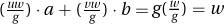 , and we are done.
By the definition of g = GCD(a, b), we know g divides a and b, and hence it divides U · a + V · b evenly. It follows that if g does not divide w evenly, then there is no integer solution to U · a + V · b = w.
4). Solution not provided.
10.4.1 1. Where in the heap can the value 1 go? It must be in one of the leaves. If 1 were not at a leaf, then the nodes below it would need a smaller number, of which there are none.
2. Which values can be stored in entry A[2]? It can contain any value in the range 7–14. It can’t contain 15, because 15 must go in A[1]. We already know that A[2] must be greater than each of the seven nodes in its subtree. Hence, it can’t contain a value less than 7. For each of the other values, a heap can be constructed such that A[2] has that value.
3. Where in the heap can the value 15 go? 15 must go in A[1] (as we have mentioned).
4. Where in the heap can the value 6 go? 6 can go anywhere except A[1], A[2], or A[3]. A[1] must contain 15, and A[2] and A[3] must be at least 7.
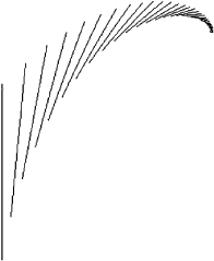
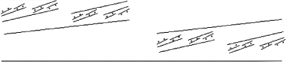
11.1.1 Falling Line: This construction consists of a single line with image n − 1 raised, tilted, and shrunk:
11.1.2 Binary Tilt: This image is the same as the birthday cake. The only differences are that the two places to recurse are tilted and one of them has be flipped upside down:
Sorry, the solution for 2 and 3 are not included.
14.2.1 The node v can’t be in Vk′ for k′ > k + 1, because there is a path of length k + 1 to it, namely the path to u followed by the edge 〈u, v,〉. If v has not been found before, then we are just finding it. Its d(v) is being set to d(u) + 1 = k + 1. By LI1, this must be its distance from s. Hence, v must be in Vk+1. If v has been found before, it is because a shortest path has already been found to it. If the edge 〈u, v,〉 is directed, then this previous path could have any length k′ ≤ k + 1. However, if this edge is undirected, then there is a catch. Suppose v is in Vk′. Then a possible path to u is that of length k′ + 1 from s to v followed by the edge {u, v,} backwards to u. because the shortest path to u is of length k, we have k′ + 1 ≥ k or k′ ∈ {k − 1, k, k + 1}.
14.2.2 The shortest-path algorithm given in this section is identical to the generic search algorithm in Section 14.1 except that a queue is used. Hence, the running time is Θ(|E|). The time is not less if you are searching for a path to a specific node t.
14.3.2 Despite differences in the algorithms, on a graph with edge weights one, breadth-first search and Dijkstra’s algorithm are identical. Breadth-first search handles the first node in its queue, whereas Dijkstra’s algorithm handles the node with the next smallest d(v). However, breadth-first search’s third loop invariant ensures that the nodes are found and added to the queue in the order of distance d(v). Hence, handling the next in the queue amounts to handling the next smallest d(v). Breadth-first search’s first loop invariant states that the correct minimal distance d(v) to v is obtained when the node v is first found, whereas with Dijkstra’s algorithm we are not sure to have it until the node is handled. However, with edge weights one, when v is first found in Dijkstra’s algorithm, d(v) is set to the length of the overall shortest path and never changed again.
14.6.2 The shortest path to node v will not contain any nodes u that appear after it in the total order, because by the requirements of the total order there is no path from u to v. Hence, it is fine to handle v, committing to a shortest path to v, before considering u. Hence, it is fine to handle the nodes in the order given by the total order. The advantage of this algorithm is that you do not need to maintain a priority queue, as done in Dijkstra’s algorithm. This decreases the time from Θ(|E| log |V|) to Θ(|E|).
15.2.5 Given a network 〈G, s, t〉, run the max flow algorithm on it. In addition to returning a maximum flow, it also returns a minimum cut, which is used to witness the fact that there is no better flow.
15.5.1 1. The first does not have a matching. A witness is the fact that nodes 1, 3, and 5 are only connected to B and D. Hence, the three can’t be matched to the two. In the language of Hall’s theorem, let A = {1, 3, 5}; then N(A) = {B, D}. Because |A| > |N(A)|, Hall’s theorem gives that there is no matching. The second does have a matching. A witness is the following matching:
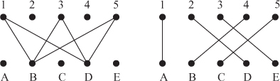
2. Consider an arbitrary A ⊆ L. Note that the set B = {M(u) | u ∈ A} contains |A| distinct nodes and that B ⊆ N(A). Hence, |A| ≤ |N(A)|.
3. Let A = U ∩ L be the set of nodes that are both on the left side of the bipartite graph and on the left side of the cut. Consider any node v ∈ N(A). Because v ∈ N(A), there is a node u ∈ A ⊂ U such that 〈u, v〉 is an edge. If v ∈ V, then this edge (u, v) crosses the cut. But this edge has capacity ∞. In this case, the capacity of the cut is well over |L|. On the other hand, if v ∈ U, then the edge from v to t is across the cut. Now consider any node u ∈ L − A ⊂ V. The edge from s to u crosses the cut. This proves that the number of edges across the cut is at least N(A) + (|L| − |A|), which by our assumption is at least |A| + (|L| − |A|) = |L|.
4. We have seen that there is a matching with |L| edges iff the max flow in this graph has value |L| iff the min cut in this graph has capacity |L|. The cut with s on one side by itself has |L| edges going across the cut, namely those edges from s to L. By the last question, if ∀A ⊆ L, |A| ≤ |N(A)|, then every cut has at least |L| edges across it. Hence, the min cut must be |L|. Hence, the max flow has value |L|. Hence, there is a matching with |L| edges. All the nodes in L must be matched.
5. By the last question, it is sufficient to prove that ∀A ⊆ L, |A| ≤ |N(A)| is true. Consider some set A ⊆ L. Because each every node in A ⊆ L has degree at least k, we know that at least k · |A| edges leave A. All of the edges that leave A must enter its neighborhood set N(A). Hence, the number that leave A is at most the number that enter N(A). Because every node in N(A) ⊆ R has degree at most k, we know that at most k · |N(A)| enter N(A). It follows that k · |A| ≤ # leave A ≤ # enter N(A) ≤ k · |N(A)|. Hence, |A| ≤ |N(A)|, as is needed.
16.2.2 In the following instance of the interval cover problem, the greedy criterion that selects the interval that covers the largest number of uncovered points would commit to the top interval. However, the optimal solution does not contain this interval, but contains the bottom two intervals.

16.3.2 Algorithms 1, 2, and 4 are suboptimal for the following counterexample instance:

Diagram (a) gives the events in the instance and the optimal schedule in two rooms. Diagram (b) gives the suboptimal schedule produced by these three algorithms. Note that the third algorithm, which schedules the next event in the room with the latest last-scheduled finishing time, gives the optimal schedule. We will now prove that it always gives an optimal solution.
As with all greedy algorithms, the loop invariant is that there is at least one optimal solution optSLI consistent with the choices made so far, that is, scheduling in the same rooms the same events whose schedule have been committed to so far and not scheduling the events rejected so far. Initially, no choices have been made, and hence trivially all optimal solutions are consistent with these choices. We prove that the loop invariant is maintained by modifying the schedule optSLI into another schedule optSours and prove that this new schedule is valid, consistent with all previous and current choices, and optimal. There are three cases.
If our greedy algorithm did not schedule the next event i, then this event must conflict in each room with a previously scheduled event. Hence, optSLI cannot have this next event i scheduled either, because it too has scheduled these previous events. Hence, optSLI itself is already consistent with the most recent choice.
If our greedy algorithm did schedule the next event i in room j and optSLI does not schedule this event at all, then we modify the schedule optSLI into optSours by adding i to room j and removing any events from j that conflict with it. Just as done with the one-room scheduling algorithm in Section 16.2.1, we can prove that only one event is removed and hence optSours is valid, consistent, and optimal.
The remaining case occurs when our greedy algorithm scheduled the next event i in room j and optSLI schedules it in room j′. (See diagram (a).) We modify the schedule optSLI into optSours as follows. (See diagram (b).) We cannot move the events whose schedule has already been committed to by the algorithm, because optSours needs to remain consistent with these choices. (See the events in the Commit circle.) We need to move event i from room j′ to room j so that it too is consistent with what the algorithm has done. But making this change may create conflicts. To fix these, we swap every event scheduled by optSLI in room j′ with the finishing time of event i or later with every such job scheduled in room j. (See the events in the rectangle.)
We now prove that the resulting solution optSours is valid, consistent, and optimal.
A Valid Solution: Our modified solution optSours contains no conflicts, because optSLI contained none and we will prove now that no new conflicts were introduced. There are no new conflicts between the previously committed events (circle), because they did not change. There are no new conflicts between the later-committed events (rectangle), because they flipped rooms all together. Event i does not conflict with the previously committed events in room j, because the algorithm scheduled it there. The even later events that were in room j′ don’t either, because they are even later. The later events that were in room j won’t conflict with the previously scheduled events in room j′, because they did not conflict with those in room j and we know by the algorithm’s choice of room j that the last-scheduled finishing time for j is later than that for room j′.
Consistent with Choices Made: optSLI was consistent with the previous choices. We moved event i from room j′ to room j to make optSours consistent with this most recent choice. We did not move any events in Commit.
Optimal: Schedule optSours has the optimal number of events in it, because it has the same number of events as optSLI.
Loop Invariant Has Been Maintained: In conclusion, we have constructed a valid optimal schedule optSours that is consistent with the choices made by the algorithm. This proves that the loop invariant has been maintained.
The rest of the proof of correctness of this greedy algorithm is the same as that of all the others.
17.5.1 Asking to provide the best word is not a “little question” for the bird. She would be doing most of the work for you. Asking the friend to provide the best place on the board to put the word is not a subinstance of the same problem as that of the given instance.
17.5.2 The simple brute force algorithm searches the dictionary for each permutation of each subset of the letters. The backtracking algorithm tries all of the possibilities for the first letter and then recurses. Each of these stack frames tries all of the remaining possibilities for the second letter, and so on. This can be pruned by observing that if the word constructed so far, e.g., ‘xq’, does not match the first letters of any word in the dictionary, then there is no need for this stack frame to recurse any further. (Another improvement on the running time ensures that the words are searched for in the dictionary in alphabetical order.)
17.5.3 1. 〈1, 5, 8, 6, 3, 7, 2, 4〉
2. 〈1, 6, 8, 3, 7, 4, 2, 5〉
3. 〈1, 7, 4, 6, 8, 2, 5, 3〉
4. 〈1, 7, 5, 8, 2, 4, 6, 3〉
5. 〈2, 4, 6, 8, 3, 1, 7, 5〉
6. 〈2, 5, 7, 1, 3, 8, 6, 4〉
7. 〈2, 5, 7, 4, 1, 8, 6, 3〉
8. 〈2, 6, 1, 7, 4, 8, 3, 5〉
9. 〈2, 6, 8, 3, 1, 4, 7, 5〉
10. 〈2, 7, 3, 6, 8, 5, 1, 4〉
11. 〈2, 7, 5, 8, 1, 4, 6, 3〉
12. 〈2, 8, 6, 1, 3, 5, 7, 4〉
17.5.4 We will prove that the running time is bounded between  and nn and hence is nΘ(n) = 2Θ(nlogn). Without any pruning, there are n choices on each of n rows as to where to place the row’s queen. This gives nn different placements of the queens. Each of these solutions would correspond to a leaf of the tree of stack frames. This is clearly an upper bound on the number when there is pruning.
I will now give a lower bound on how many stack frames will be executed by this algorithm. Let j be one of the first  rows. I claim that each time that a stack frame is placing a queen on this row, it has at least
  choices as to where to place it. The stack frame can place the queen on any of the n squares in the row as long as this square cannot be captured by one of the queens placed above it. If row i is above our row j, then the queen placed on row i can capture at most three squares of row j: one by moving on a diagonal to the left, one by moving straight down, and one by moving on a diagonal to the right. Because j is one of the first rows, there are at most this number of rows i above it, and hence at most
  of row j’s squares can be captured. This leaves, as claimed, squares on which the stack frame can place the queen.
From the above claim, it follows that within the tree of stack frames, each stack frame within the tree’s first levels branches out to at least children. Hence, at the  th level of the tree there are at least different stack frames. Many of these will terminate without finding a complete valid placement. However, this is a lower bound on the running time of the algorithm, because the algorithm recurses to each of them.
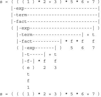
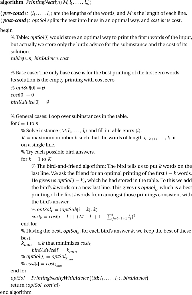
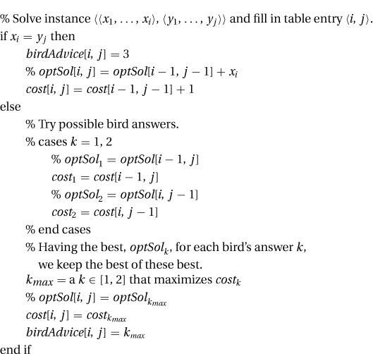
17.5.5 The line “kmin = a k that maximizes costk.”
19.1.1 (a): If xn = ym, then we must prove that there is at least one optimal solution that contains both of these last characters. Consider an optimal solution. It must end in this last character; otherwise it could be extended to contain it. It might not contain both of them, as in the case of X = 〈A, B, B〉, Y = 〈A, B〉, with optimal solution Z = 〈A, B〉. However, as in this case, we can just as well assume that the optimal solution takes both. If xn ≠ ym, then the optimal solution cannot take both. Hence, it either does not take the last of X or does not take the last of Y. It might not take the last of either, but this is included in both the other two cases. See Section 17.3 for a further answer.
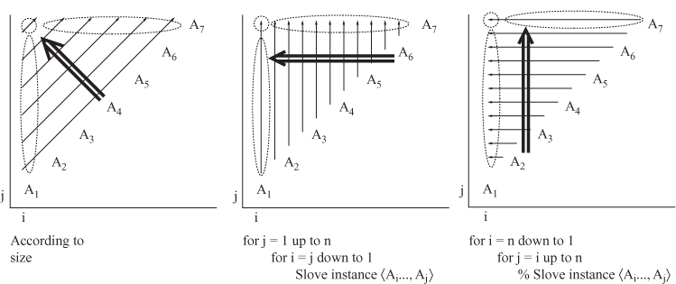
(b) The loop over subinstances is then changed as follows.
19.1.2 The running time is the number of subinstances times the number of possible bird answers, and the space is the number of subinstances. The number of subinstances is Θ(n2), and the bird has K = 3 possible answers for you. Hence, the time and space requirements are both Θ(n2).
19.5.1 1. An AVL tree of height h has left and right subtrees of heights either 〈h − 2, h − 1〉, 〈h − 1, h − 1〉, or 〈h − 1, h − 2〉.
2. The bird tells me whether the subtree heights are 〈h − 2, h − 1〉, 〈h − 1, h − 1〉, or 〈h − 1, h − 2〉. She also tells me which value ak will be at the root. I can then ask the friends for the best left and right subtrees of the specified height.
3. In each of these three cases, the heights are within 1.
4. The complete set of subinstances is as following. Recall that in Chapter 10 we proved that the minimum height of an AVL tree with n nodes is h = log2 n and that its maximum height is h = 1.455 log2 n. Hence, the complete set of subinstances is S = {〈h; ai, … , aj; pi, … , pj〉 | 1 ≤ i ≤ j ≤ n, h ∈ [log2(j − i + 1)..1.455 log2 (j − i + 1)]}. The table is a three-dimensional Θ(n × n × log n) box.
5. The table has size Θ(n × n × log n). The bird can give 3 · n different answers. Hence, the running time is Θ(n3 log n).
6. In the original problem, the height was not fixed. To solve this problem, we could simply run the previous algorithm for each h and take the best of the resulting AVL trees. However, after running the previous algorithm once, the table already contains the cost of the best AVL for each of the possible heights h. To find the best overall AVL tree, we need only compare those listed in the table.
Time and space requirements: The running time is the number of subinstance times the number of possible bird answers, and the space is the number of subinstances. The number of subinstances indexing your table is Θ(|V|n2), namely, Table[h, i, j] for h ∈ V and 1 ≤ i ≤ j ≤ n. The number of answers that the bird might give you is at most O(mn), namely, 〈q, k〉 for each of the m rules rq and the split k ∈ [1..n − 1]. This gives time = O(|V|n2 · mn). If the grammar G is fixed, then the time is Θ(n3).
A tighter analysis would note that the bird would only answer q for rules rq = “Aq ⇒ BqCq", for which the left-hand side Aq is the nonterminal Th specified in the instance. Let  be the number of such rules. Then the loop over nonterminals Th and the loop over rules rq would not require |V|m time, but
  . This gives a total time of Θ(n3m).
19.8.2 Given an instance E = {e1, e2, … , en} of the elephant problem, we map this to an instance 〈X, Y〉 of the LCS problem as follows. Each elephant will be distinct. Let X = 〈x1, … , xn〉 be the elephants sorted by weight wi, and let Y = 〈y1, … , ym〉 be the same sorted by smartness si. A solution to LCS is a subsequence Z = 〈z1, … , zl〉 that is common to both X and Y. Note that Z is a subset of elephants S ⊆ E for which bigger is smarter. This is because Z is sorted both with respect to weight and with respect to intelligence. The only difference between these problems is that the cost (or success) of a LCS solution is simply the length of Z, while for the elephant problem it is the sum of the values of the elephants. Hence, for this to work, the LCS problem needs to be generalized to have weights on the letters. But this would not change the dynamic programming algorithm at all.
20.2.4 The first is easy. InstanceMap(I1) simply maps each instance I1 ∈ S1 ⊆ S2 of P1 to itself, I1, which is a valid instance of P2. The second is much harder, because InstanceMap(I2) must map each instance I2 ∈ S2 of P2 to some instance I1 within the restricted set S1.
20.2.5 The running time Time(Algoracle) is measured as a function of its own input size, namely  . But because |Ioracle| = |Ialg|2, this same time is
  , in terms of Algalg’s input size. The extra O(|Ialg|3) time for the mappings is not substantial. Hence, Algalg’s total running time is
  .
.
Similarly, if Algoracle runs in polynomial time, namely Time(Algoracle) = Θ(| Ioracle|c), then so does Algalg, namely Time(Algalg) = Θ(|Ialg|2c + |Ialg|3), but note that the polynomal is a different one.
Step 5: Given a graph GCOL that we want to color, we construct an instance 〈GInd, NInd〉 = InstanceMap(GCOL) to give to the independent set oracle as follows. As said, GInd will have a node for each pair 〈u, c〉 where u is a node of GCOL and c is one of the three colors. For each node u ∈ GCOL, we put a triangle of edges around 〈u, red〉, 〈u, blue〉, and 〈u, green〉. For each edge 〈u, v〉 ∈ GCOL, we put three parallel edges between 〈u, c〉 and 〈v, c〉, for each color c. The size of the required independent set will be the number of nodes, NInd = |VCOL|, in the graph GCOL.
Step 6: Given an independent-set solution SInd to GInd of size | VCOL|, we construct a coloring SCOL for GCOL by coloring u with color c if node 〈u, c〉 is in the independent set.
Step 7: We now show that if SInd is a valid independent set of size |VCOL|, then SCOL is a valid 3-coloring. First we show that it is impossible for a node to be given more than one color, because the edge between 〈u, c〉 and 〈u, c′〉 prevents both of these nodes being in the independent set. Because the independent set is of size |VCOL| and no node u appears more than once, it follows that every node u appears exactly once. Hence, every node u is given a color. Finally, we show that the nodes in the edge 〈u, v〉 ∈ GCOL cannot both have the color c, because the edge between 〈u, c〉 and 〈v, c〉 prevents both of these nodes from being in the independent set.
Step 8: Given a coloring SCOL, for GCOL, we construct an independent set SInd for GInd of size |VCOL| by putting node 〈u, c〉 in the independent set if u is colored c.
Step 9: We now show that if SCOL is a valid 3-coloring, then SInd is a valid independent set. We need to show that for each edge in GInd, both nodes are not in SInd. There is an edge between 〈u, c〉 and 〈u, c′〉, but u cannot have both colors c and c′. There is an edge between 〈u, c〉 and 〈v, c〉, but u and v cannot both have color c.
22.0.2 1. ∀x ∃y x + y = 5 is true. Let x have an arbitrary real value, and let y = 5 − x. Then x + y = 5.
2. ∃y ∀x x + y = 5 is false. Let y have an arbitrary real value, and let x = 6 − y. Then x + y ≠ 5.
3. ∀x ∃y x · y = 5 is false. Let x = 0. Then y must be  , which is impossible.
4. ∃y ∀x x · y = 5 is false. Let y have an arbitrary real value, and let  if y ≠ 0 and x = 0 if y = 0. Then x · y ≠ 5.
5. ∀x ∃y x · y = 0 is true. Let x have an arbitrary real value, and let y = 0. Then x · y = 0.
6. ∃y ∀x x · y = 0 is true. Let y = 0, and let x have an arbitrary real value. Then x · y = 0.
7. [∀x ∃y P(x, y)] ⇒ [∃y ∀x P(x, y)] is false. Let P(x, y) = [x + y = 5]. Then, as already seen, the first is true and the second is false.
8. [∀x ∃y P(x, y)] ⇐ [∃y ∀x P(x, y)] is true. Assume the right side is true. Let y0 be the y for which [∀x P(x, y)] is true. We prove the left side as follows. Let x have an arbitrary real value, and let y = y0. Then P(x, y0) is true.
9. Sorry, not provided.
23.1.1 The number of operations is T = 24 × 60 × 60 × 106 = 8.64 × 10¹⁰. We have  .
.
23.1.4 1. We first prove that g + h = Θ(max(g, h)) as follows. max(g, h) ≤ g + h, assuming that both g and h are positive and g + h ≤ 2 max(g, h).
2. One can set k to absolutely minimize f(n, k) by setting f's derivative wrt k equal to zero and solving for k. Sometimes this is hard. Because  and we do not care about the multiplicative constant, let us instead set k in order to minimize
  . Observe that if k is very small, then the first term, being very big, dominates. Hence, we can make the whole expression smaller by increasing k. Similarly, if k is big, the second term dominates the expression, and we can decrease it by decreasing k. So for the optimal solution the two terms should be roughly the same. In this case
  gives n = k and
  . This is (asymptotically) the best result, because decreasing k increases the first term and increasing k increases the second.
3. Sorry, not included.
23.2.1 1. ∃A, ∀I, Works(Sorting, A, I). We know that there at least one algorithm, e.g., A = merge sort, that works for every input instance I.
2. ∀A, ∃I, ¬ Works(Halting, A, I) We know that contrary statement is true. Every algorithm fails to work for at least one input instance I.
3. ∃P, ∀A, ∃I, ¬ Works(P, A, I)
4. It says that every input has some algorithm that happens to output the right answer. It is true. Consider an arbitrary instance I. If on instance I, Halting happens to say yes, then let A be the algorithm that simply halts and says yes. Otherwise, let A be the algorithm that simply halts and says no. Either way, A works for this instance I.
5. It says that every algorithm correctly solves some problem. This is not true, because some algorithms do not halt on some input instances. We prove the complement ∃A, ∀P, ∃I, ¬Works(P, A, I) as follows. Let A be an algorithm that runs forever on some instance I′. Let P be an arbitrary problem. Let I be an instance I′ on which A does not halt. Note that Works(P, A, I) is not true.
25.1.4 Exercise 25.0.2 proves that 3log n < < n for sufficiently big n. Hence, n2 ≤ 3n2 logn ≤ n · n2 = n3.
1. 14n9 + 5, 000n7 + 23n2 log n ∈ O(n9): Let c = 15 and n0 = 100. For all n ≥ 100, We have  .
.
2. 2n2 − 100n ∈ Θ(n2): Let c1 = 1, c2 = 2, and n0 = 100. For all n ≥ 100, c1 g(n) = 1n2 = 2n2 − n · n ≤ 2n2 − 100n = f(n) ≤ 2n2 = c2g(n).
3. 14n8 − 100n6 ∉ O(n7): Let c and n0 be arbitrary values given to us by some adversary. We then let n = max(10, c, n0). Then we demonstrate that f(n) is too big. Because n ≥ 10, we have 100n6 ≤ n8. This gives f(n) = 14n8 − 100n6 ≥ 14n8 − 1n8 > n · n7 ≥ c · n7.
4. 14n8 + 100n6 ∉ Θ(n9): Let c1, c2, and n0 be arbitrary values given to us by some adversary. Let us make n = max(15/c1, 11, n0). Then we demonstrate that f(n) is too small:  .
.
5. 2n+1 ∈ O(2n): Let c = 2 and n0 = 0. For all n ≥ 0, f(n) = 2n+1 ≤ 2 × 2n = c × g(n).
6. 22n ∉ O(2n): Let c and n0 be arbitrary values. Let n = max(1 + log2 c, n0). Then we have that f(n) = 22n = 2n · 2n > c · g(n).
1. x = 7y3(log2 y)18 ∈ y3+o(1) = [y3, y3+ε]. Solving this gives y = x1/(3+o(1)).
2. Substituting in y = x1/3+o(1) gives x = 7y3(log2 y)18 = 7 y3(log2 x1/(3+o(1)))18 = Θ(y3(log2 x)18). Solving this gives  .
.
26.2.1 His first such step takes him half an hour, his second a quarter, his third an eighth, … for a total of only  hour. Given that he travels one kilometer at one kilometer an hour, this is reasonable.
1. The function  is 2Ω(n), because it is bounded between 2n and 22n. Let n = 2k. Then ⌈log2 n⌉ = k and
  , but for n′ = n + 1 we have ⌈log n′⌉ = k + 1 and
  .
.
2. We show  as follows. With n = 2k, both functions are more or less constant from
  to f(n). Because they behave like arithmetic functions within this range, the adding-made-easy techniques give that
  and not Θ(f(n)).
3. We show that  by bounding it between
  and n. Let
  . Then ⌊loglog n⌋ = k and
  , but for n′ = n − 1 we have ⌊loglog n′⌋ = k − 1 and
  .
.
4. We show that  as follows. Again let , so that f(n) = n, yet every previous term is most . The total of
  then is at most
  . Because the last term f(n) is so much bigger than the previous ones, the total is not Θ(n · f(n)), which is Θ(n2).
5. The function  is a geometric counterexample squeezed between 2n and 22n, just as
  is:
is:
27.1.1 Examples:
27.2.1 Plugging Fib(n) = αn into Fib(n) = Fib(n − 1) + Fib(n − 2) gives that αn = αn−1 + αn−2. Dividing through by αn−2 gives α2 = α + 1. Solving this gives that either  or
or  . Any linear combination of these two solutions will also be a valid solution, namely Fib(n) = c1 · (α1)n + c2 · (α2)n. Using the fact that Fib(0) = 0 and Fib(1) = 1 and solving for c1 and c2 gives that
27.2.2 Unwinding:
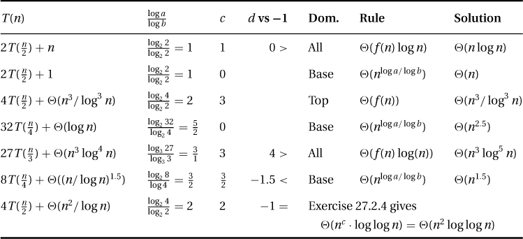
1. T(n) = T(n−1) + n: Because a = 1 and c > 1, the table give T(n) = Θ(n · f(n)) = Θ(n2). Unwinding gives T(n) = n + T(n−1) = n + (n−1) + T(n−2) = n + (n−1) + (n−2) + T(n−3) = n + (n−1) + (n−2) + · · · + (n−i + 1) + T(n−i) = n + (n−1) + (n−2) + · · · + 1 = Θ(n2).
2. T(n) =2 · T(n − 1) + 1: Because a = 2, the table gives  . Unwinding gives T(n) = 1 + 2T(n−1) = 1 + 2 + 4T(n−2) = 1 + 2 + 4 + · · · + 2i−1 + 2iT(n−i) = 1 + 2 + 4 + · · · + 2n−1 + 2n = Θ(2n).
27.2.4 Suppose f(n) = nc · logd n and  ; then
  . The expression n/bi takes on the values n, n/b, n/b2, … , 1. Reversing this order gives
  . Here [logb]d is a constant that we can hide in the Theta. This gives
 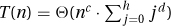 . The adding-made-easy approximations state that this sum is arithmetic as long as d > −1. In this case, the total is T(n) = Θ(nc · h · hd) = Θ(nc · logd+1 n) = Θ(f(n) logn). If d = −1, then we get the harmonic sum
  . If d < −1, then the sum has a bounded tail, giving T(n) = Θ(nc · Θ(1)) = Θ(nloga/logb).

 .
.