The brute force algorithm for an optimization problem is to simply compute the cost or value of each of the exponential number of possible solutions and return the best. A key problem with this algorithm is that it takes exponential time. Another (not obviously trivial) problem is how to write code that enumerates over all possible solutions. Often the easiest way to do this is recursive backtracking. The idea is to design a recurrence relation that says how to find an optimal solution for one instance of the problem from optimal solutions for some number of smaller instances of the same problem. The optimal solutions for these smaller instances are found by recursing. After unwinding the recursion tree, one sees that recursive backtracking effectively enumerates all options. Though the technique may seem confusing at first, once you get the hang of recursion, it really is the simplest way of writing code to accomplish this task. Moreover, with a little insight one can significantly improve the running time by pruning off entire branches of the recursion tree. In practice, if the instance that one needs to solve is sufficiently small and has enough structure that a lot of pruning is possible, then an optimal solution can be found for the instance reasonably quickly. For some problems, the set of subinstances that get solved in the recursion tree is sufficiently small and predictable that the recursive backtracking algorithm can be mechanically converted into a quick dynamic programming algorithm. See Chapter 18. In general, however, for most optimization problems, for large worst case instances, the running time is still exponential.
An Algorithm as a Sequence of Decisions: An algorithm for finding an optimal solution for your instance must make a sequence of small decisions about the solution: “Do we include the first object in the solution or not?” “Do we include the second?” “The third?”…, or “At the first fork in the road, do we go left or right?” “At the second fork which direction do we go?” “At the third?”…. As one stack frame in the recursive algorithm, our task is to deal only with the first of these decisions. A recursive friend will deal with the rest. We saw in Chapter 16 that greedy algorithms make decisions simply by committing to the option that looks best at the moment. However, this usually does not work. Often, in fact, we have no inspirational technique to know how to make each decision in a way that leads to an optimal (or even a sufficiently good) solution. The difficulty is that it is hard to see the global consequences of the local choices that we make. Sometimes a local initial sacrifice can globally lead to a better overall solution. Instead, we use perspiration. We try all options.
EXAMPLE 17.1.1 Searching a Maze
When we come to a fork in the road, all possible directions need to be tried. For each, we get a friend to search exhaustively, backtrack to the fork, and report the highlights. Our task is to determine which of these answers is best overall. Our friends will have their own forks to deal with. However, it is best not to worry about this, since their path is their responsibility, not ours.
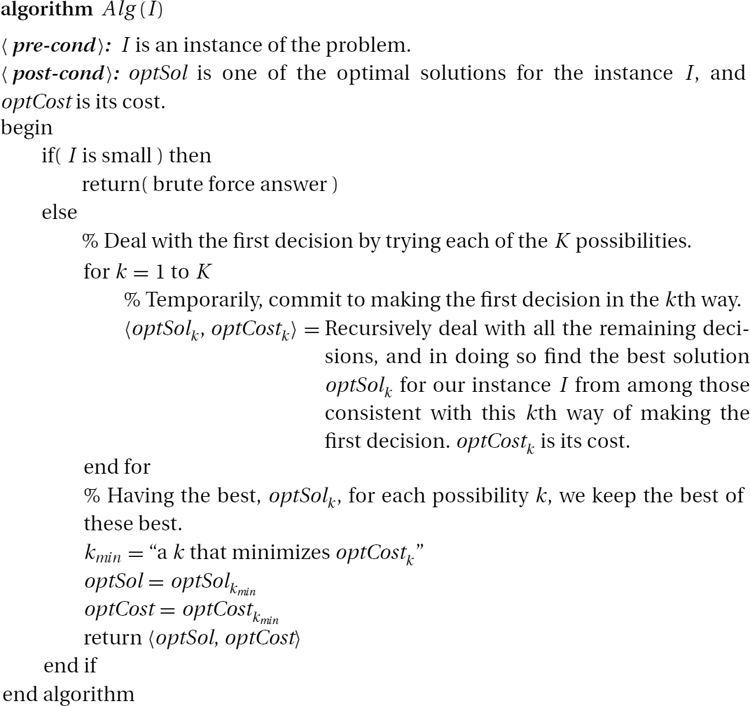
High-Level Code: The following is the basic structure that the code will take.
EXAMPLE 17.1.2 Searching for the Best Animal
Suppose, instead of searching through a structured maze, we are searching through a large set of objects, say for the best animal at the zoo. See Figure 17.1. Again we break the search into smaller searches, each of which we delegate to a friend. We might ask one friend for the best vertebrate and another for the best invertebrate. We will take the better of these best as our answer. This algorithm is recursive. The friend with the vertebrate task asks a friend to find the best mammal, another for the best bird, and another for the best reptile.
A Classification Tree of Solutions: This algorithm unwinds into the tree of stack frames that directly mirrors the taxonomy tree that classifies animals. Each solution is identified with a leaf.
Iterating through the Solutions to Find the Optimal One: This algorithm amounts to using depth-first search (Section 14.4) to traverse this classification tree, iterating through all the solutions associated with the leaves. Though this algorithm may seem complex, it is often the easiest way to iterate through all solutions.
Speeding Up the Algorithm: This algorithm is not any faster than the brute force algorithm that simply compares each animal with every other. However, the structure that the recursive backtracking adds can possibly be exploited to speed up the algorithm. A branch of the tree can be pruned off when we know that this does not eliminate all optimal solutions. Greedy algorithms (Chapter 16) prune off all branches except one path down the tree. In Section 18.2, we will see how dynamic programming reuses the optimal solution from one subtree within another subtree.
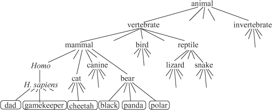
Figure 17.1: Classification tree of animals.
The Little Bird Abstraction: I like to use a little bird abstraction to help focus on two of the most difficult and creative parts of designing a recursive backtracking algorithm.
What Question to Ask: The key difference between searching a maze and searching for the best animal is that in the first the forks are fixed by the problem, but in the second the algorithm designer is able to choose them. Instead of forking on vertebrates vs invertebrates, we could fork on brown animals vs green animals. This choice is a difficult and creative part of the algorithm design process. It dictates the entire structure of the algorithm, which in turns dictates how well the algorithm can be sped up. I like to view this process of forking as asking a little bird a question, “Is the best animal a vertebrate or an invertebrate?” or “Is the best vertebrate, a mammal, a bird, a reptile, or a fish?” The classification tree becomes a strategy for the game of twenty questions. Each sequence of possible answers (for example, vertebrate–mammal–cat–cheetah) uniquely specifies an animal. Worrying only about the top level of recursion, the algorithm designer must formulate one small question about the optimal solution that is being searched for. The question should be such that having a correct answer greatly reduces your search.
Constructing a Subinstance for a Friend: The second creative part of designing a recursive backtracking algorithm is how to express the problem “Find the best mammal” as a smaller instance of the same search problem. The little bird helps again. We pretend that she answered “mammal.” Trusting (at least temporarily) in her answer helps us focus on the fact that we are now only considering mammals, and this helps us to design a subinstance that asks for the best one. A solution to this subinstance needs to be translated before it is in the correct form to be a solution to our instance.
A Flock of Stupid Birds vs. a Wise Little Bird: The following two ways of thinking about the algorithm are equivalent.
A Flock of Stupid Birds: Suppose that our question about whether the optimal solution is a mammal, a bird, or a reptile has K different answers. For each, we pretend that a bird gave us this answer. Giving her the benefit of doubt, we ask a friend to give us the optimal solution from among those that are consistent with this answer. At least one of these birds must have been telling us the truth. We find it by taking the best of the optimal solutions obtained in this way. See Figure 17.2 for an illustration of these ideas.
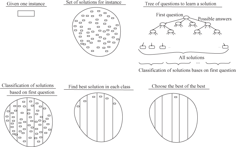
Figure 17.2: Classifying solutions and taking the best of the best.
A Wise Little Bird: If we had a little bird who would answer our questions correctly, designing an algorithm would be a lot easier: We ask the little bird “Is the best animal a bird, a mammal, a reptile, or a fish?” She tells us a mammal. We ask our friend for the best mammal. Trusting the little bird and the friend, we give this as the best animal. Just as nondeterministic finite automata (NFAs) and nondeterministic Turing machines can be viewed as higher powers that provide help, our little bird can be viewed as a limited higher power. She is limited in that we can only ask her questions that do not have too many possible answers, because in reality we must try all these possible answers.
This section presents the steps that I recommend using when developing a recursive backtracking algorithm. To demonstrate them, we will develop an algorithm for the queens problem.
EXAMPLE 17.2.1 The Queens Problem
Physically get yourself (or make on paper) a chessboard and eight tokens to act as queens. More generally, you could consider an n × n board and n queens. A queen can move as far as she pleases, horizontally, vertically, or diagonally. The goal is to place all the queens on the board in a way such that no queen is able to capture any other.
Try It: Before reading on, try yourself to place the queens on an 8-by-8 board. How would you do it?
1) Specification: The first step is to be very clear about what problem needs to be solved. For an optimization problem, we need to be clear about what the set of instances is; for each instance, what its set of solutions is; and for each solution, what its cost or value is.
Queens: The set of possible solutions is the set of ways placing the queens on the board. We do not value one solution over another as long as it is valid, i.e., no queen is able to capture any other queen. Hence, the value of a solution can simply be one if it is a valid solution and zero if not. What is not clear is what an input instance for this problem is, beyond the dimension n. We will need to generalize the problem to include more instances in order to be able to recurse. However, we will get back to that later.
2) Design a Question and Its Answers for the Little Bird: Suppose the little bird knows one of the optimal solutions for our instance. You, the algorithm designer, must formulate a small question about this solution and the list of its possible answers.
Question about the Solution: The question should be such that having a correct answer greatly reduces the search. Generally, we ask for the first part of the solution.
Queens: We might ask the bird, “Where should I place the first queen?”
The Possible Bird Answers: Together with your question, you provide the little bird with a list A1, A2,…, AK of possible answers, and she simply returns the index k ∈ [1..K] of her answer. To be consistent, we will always use the letter k to index the bird answers. In order for the final algorithm to be efficient, it is important that the number K of different answers be small.
Queens: Given that there are n queens and n rows and that two queens cannot be placed in the same row, the first observation is that the first queen must be in the first row. Hence, there are K = n different answers the bird might give.
3) Constructing Subinstances: Suppose that the bird gives us the kth of her answers. This giving us some of the solution; we want to ask a recursive friend for the rest of the solution. The friend must be given a smaller instance of the same search problem. You must formulate subinstance subI for the friend so that he returns to us the information that we desire.
Queens: I start by (at least temporarily) trusting the bird, and I place a queen where she says in the first row. In order to give an instance to the friend, we need to go back to step 1 and generalize the problem. An input instance will specify the locations of queens in the first r rows. A solution is a valid way of putting the queens in the remaining rows. Given such an instance, the question for the bird is “Where does the queen in the next row go?” Trusting the bird, we place a queen where she says. The instance, subI, we give the friend is the board with these r + 1 queens placed.
Trust the Friend: We proved in Section 8.7 that we can trust the friend to provide an optimal solution to the subinstance subI, because he is really a smaller recursive version of ourselves.
4) Constructing a Solution for My Instance: Suppose that the friend gives you an optimal solution optSubSol for his instance subI. How do you produce an optimal solution optSol for your instance I from the bird’s answer k and the friend’s solution optSubSol?
Queens: The bird tells you where on the r + 1st row the queen should go and your friend tells you where on the rows r + 2 to n the queens should go. Your solution combines these to tell where the on the rows r + 1 to n the queens should go.
We can trust the friend to give provide an optimal solution to the subinstance subI, because he is really a smaller recursive version of ourselves. Recall, in Section 8.7, we used strong induction to prove that we can trust our recursive friends.
5) Costs of Solutions and Subsolutions: We must also return the cost optCost of our solution optSol.
Queens: The solutions in this case, don’t have costs.
6) Best of the Best: Try all the bird’s answers, and take best of the best.
Queens: If we trust both the bird and the friend, we conclude that this process finds us a best placement of the queens. If, however, our little bird gave us the wrong placement of the queen in the r + 1st row, then this might not be the best placement. However, our work was not wasted, because we did succeed in finding the best placement from amongst those consistent with this bird’s answer. Not trusting the little bird, we repeat this process, finding a best placement starting with each of the possible bird answers. Because at least one of the bird answers must be correct, one of these placements must be an overall best. We return the best of these best as the overall best placement.
To find the best of these best placements, let optSolk and optCostk denote the optimal solution for our instance I and its cost that we formed when temporarily trusting the kth bird’s answer. Search through this list of costs optCost1, optCost2,…, optCostK, finding the best one. Denote the index of the chosen one by kmax. The optimal solution that we will return is then 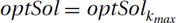 and its cost is
 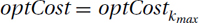 .
.
7) Base Cases: The base case instances are instances of your problem that are small enough that they cannot be solved using steps 2–6, but they can be solved easily in a brute force way. What are these base cases, and what are their solutions?
Queens: If all n queens have been placed, then there is nothing to be done.
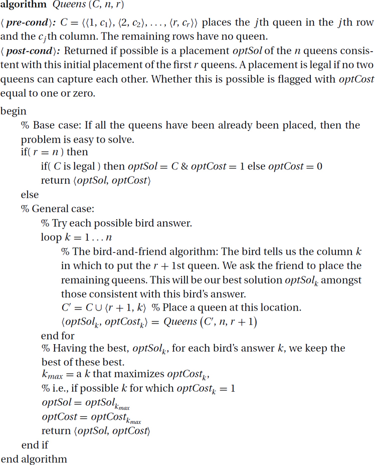
8) Code: The following code might be made slightly simpler, but in order to be consistent we will always use this same basic structure.
9) Recurrence Relations: At the core of every recursive backtracking and dynamic programming algorithm is a recurrence relation. These define one element of a sequence as a function of previous elements in the same sequence. The following are examples.
The Fibonacci Sequence: If Fib(i) is the ith element in the famous Fibonacci sequence, then Fib(n) = Fib(n − 1) + Fib(n − 2). The base cases Fib(0) = 0 and Fib(1) = 1 are also needed.
Running Time: If T(n) is the running time of merge sort on an input of n numbers, then we have 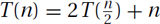 . The base case T(1) = 1 is also needed.
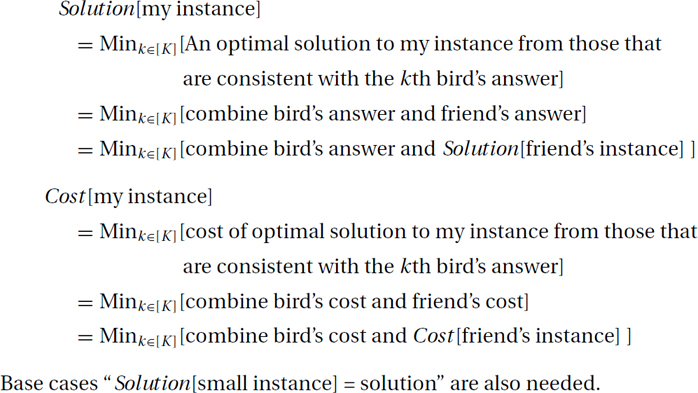
Optimal Solution: Suppose Solution[I] is defined to be an optimal solution for instance I of a problem, and Cost[I] is its cost. This is not a sequence of elements like the previous examples, because I is not in integer. However, in Chapter 18 the instances will be indexed by integers i so that Solution[i] and Cost[i] are sequences. But even when I is an arbitrary input instance, a recurrence relation can be developed as follows from the bird – friend algorithm.
Queens: For our queens example this becomes

This is bit of a silly example, because here all the work is done in the base cases.
Running Time: A recursive backtracking algorithm faithfully enumerates all solutions for your instance and hence requires exponential time. We will see that this time can be reduced by pruning off branches of the recursion tree.
The following are typical reasons why an entire branch of the solution classification tree can be pruned off.
Invalid Solutions: Recall that in a recursive backtracking algorithm, the little bird tells the algorithm something about the solution and then the algorithm recurses by asking a friend a question. Then this friend gets more information about the solution from his little bird, and so on. Hence, following a path down the recursive tree specifies more and more about a solution until a leaf of the tree fully specifies one particular solution. Sometimes it happens that partway down the tree, the algorithm has already received enough information about the solution to determine that it contains a conflict or defect making any such solution invalid. The algorithm can stop recursing at this point and backtrack. This effectively prunes off the entire subtree of solutions rooted at this node in the tree.
Queens: Before we try placing a queen on the square  r + 1, k
 , we should check to make sure that this does not conflict with the locations of any of the queens on 1, c1, 2, c2,…, r, cr. If it does, we do not need to ask for help from this friend. Exercise 17.5.4 bounds the resulting running time.
Time Saved: The time savings can be huge. Recall that for Example 9.2.1 in Section 9.2, reducing the number of recursive calls from two to one decreased the running time from Θ(N) to Θ(log N), and how in Example 9.2.2 reducing the number of recursive calls from four to three decreased the running time from Θ(n2) to Θ(n1.58…).
No Highly Valued Solutions: Similarly, when the algorithm arrives at the root of a subtree, it might realize that no solutions within this subtree are rated sufficiently high to be optimal—perhaps because the algorithm has already found a solution provably better than all of these. Again, the algorithm can prune this entire subtree from its search.
Greedy Algorithms: Greedy algorithms are effectively recursive backtracking algorithms with extreme pruning. Whenever the algorithm has a choice as to which little bird’s answer to take, i.e., which path down the recursive tree to take, instead of iterating through all of the options, it goes only for the one that looks best according to some greedy criterion. In this way the algorithm follows only one path down the recursive tree. Greedy algorithms are covered in Chapter 16.
Modifying Solutions: Let us recall why greedy algorithms are able to prune, so that we can use the same reasoning with recursive backtracking algorithms. In each step in a greedy algorithm, the algorithm commits to some decision about the solution. This effectively burns some of its bridges, because it eliminates some solutions from consideration. However, this is fine as long as it does not burn all its bridges. The prover proves that there is an optimal solution consistent with the choices made by modifying any possible solution that is not consistent with the latest choice into one that has at least as good value and is consistent with this choice. Similarly, a recursive backtracking algorithm can prune of branches in its tree when it knows that this does not eliminate all remaining optimal solutions.
Queens: By symmetry, any solution that has the queen in the second half of the first row can be modified into one that has the this queen in the first half, simply by flipping the solution left to right. Hence, when placing a queen in the first row, there is no need to try placing it in the second half of the row.
Depth-First Search: Recursive depth-first search (Section 14.5) is a recursive backtracking algorithm. A solution to the optimization problem of searching a maze for cheese is a path in the graph starting from s. The value of a solution is the weight of the node at the end of the path. The algorithm marks nodes that it has visited. Then, when the algorithm revisits a node, it knows that it can prune this subtree in this recursive search, because it knows that any node reachable from the current node has already been reached. In Figure 14.9, the path s, c, u, v is pruned because it can be modified into the path s, b, u, v, which is just as good.
A famous optimization problem is called satisfiability, or SAT for short. It is one of the basic problems arising in many fields. The recursive backtracking algorithm given here is referred to as the Davis–Putnam algorithm. It is an example of an algorithm whose running time is exponential for worst case inputs, yet in many practical situations can work well. This algorithm is one of the basic algorithms underlying automated theorem proving and robot path planning, among other things.
The Satisfiability Problem:
Instances: An instance (input) consists of a set of constraints on the assignment to the binary variables x1, x2,…, xn. A typical constraint might be 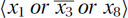 , meaning (x1 = 1 or x3 = 0 or x8 = 1) or equivalently that either x1 is true, x3 is false, or x8 is true. More generally an instance could be a more general circuit built with AND, OR, and NOT gates, but we leave this until Section 20.1.
Solutions: Each of the 2n assignments is a possible solution. An assignment is valid for the given instance if it satisfies all of the constraints.
Measure of Success: An assignment is assigned the value one if it satisfies all of the constraints, and the value zero otherwise.
Goal: Given the constraints, the goal is to find a satisfying assignment.
Iterating through the Solutions: The brute force algorithm simply tries each of the 2n assignments of the variables. Before reading on, think about how you would nonrecursively iterate through all of these solutions. Even this simplest of examples is surprisingly hard.
Nested Loops: The obvious algorithm is to have n nested loops each going from 0 to 1. However, this requires knowing the value of n before compile time, which is not likely.
Incrementing Binary Numbers: Another option is to treat the assignment as an n-bit binary number and then loop through the 2n assignments by incrementing this binary number each iteration.
Recursive Algorithm: The recursive backtracking technique is able to iterate through the solutions with much less effort in coding. First the algorithm commits to assigning x1 = 0 and recursively iterates through the 2n−1 assignments of the remaining variables. Then the algorithm backtracks, repeating these steps with the choice x1 = 1. Viewed another way, the first little bird question about the solutions is whether the first variable x1 is set to zero or one, the second question asks about the second variable x2, and so on. The 2n assignments of the variables x1, x2,…, xn are associated with the 2n leaves of the complete binary tree with depth n. A given path from the root to a leaf commits each variable xi to being either zero or one by having the path turn to either the left or to the right when reaching the ith level.
Instances and Subinstances: Given an instance, the recursive algorithm must construct two subinstances for its friends’ to recurse with. There are two techniques for doing this.
Narrowing the Class of Solutions: Associated with each node of the classification tree is a subinstance defined as follows: The set of constraints remains unchanged except that the solutions considered must be consistent in the variables x1, x2,…, xr with the assignment given by the path to the node. Traversing a step further down the classification tree further narrows the set of solutions.
Reducing the Instance: Given an instance consisting of a number of constraints on n variables, we first try assigning x1 = 0. The subinstance to be given to the first friend will be the constraints on remaining variables given that x1 = 0. For example, if one of our original constraints is 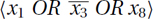 , then after assigning x1 = 0, the reduced constraint will be
  . This is because it is no longer possible for x1 to be true, given that one of
  or x8 must be true. On the other hand, after assigning x1 = 1, the original constraint is satisfied independently of the values of the other variables, and hence this constraint can be removed.
Pruning: This recursive backtracking algorithm for SAT can be sped up. This can either be viewed globally as a pruning off of entire branches of the classification tree or be viewed locally as seeing that some subinstances, after they have been sufficiently reduced, are trivial to solve.
Pruning Branches Off the Tree: Consider the node of the classification tree arrived at down the subpath x1 = 0, x2 = 1, x3 = 1, x4 = 0,…, x8 = 0. All of the assignment solutions consistent with this partial assignment fail to satisfy the constraint 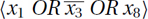 . Hence, this entire subtree can be pruned off.
Trivial Subinstances: When the algorithm tries to assign x1 = 0, the constraint is reduced to  . Assigning x2 = 1 does not change this particular constraint. Assigning x3 = 1 reduces this constraint further to simply x8, stating that x8 must be true. Finally, when the algorithm is considering the value for x8, it sees from this constraint that x8 is forced to be one. Hence, the x8 = 1 friend is called, but the x8 = 0 friend is not.
Stop When an Assignment is Found: The problem specification only asks for one satisfying assignment. Hence, the algorithm can stop when one is found.
Davis–Putnam: The above algorithm branches on the values of each variable, x1, x2,…, xn, in order. However, there is no particular reason that this order needs to be fixed. Each branch of the recursive algorithm can dynamically use some heuristic to decide which variable to branch on next. For example, if there is a variable, like x8 in the preceding example, whose assignment is forced by some constraint, then clearly this assignment should be done immediately. Doing so removes this variable from all the other constraints, simplifying the instance. Moreover, if the algorithm branched on x4,…, x7 before the forcing of x8, then this same forcing would need to be repeated within all 24 of these branches.
If there are no variables to force, a common strategy is to branch on the variable that appears in the largest number of constraints. The thinking is that the removal of this variable may lead to the most simplification of the instance.
An example of how different branches may set the variables in a different order is the following. Suppose that x1 OR x2 and  are two of the constraints. Assigning x1 = 0 will simplify the first constraint to x2 and remove the second constraint. The next step would be to force x2 = 1. On the other hand, assigning x1 = 1 will simplify the second constraint to forcing x3 = 1.
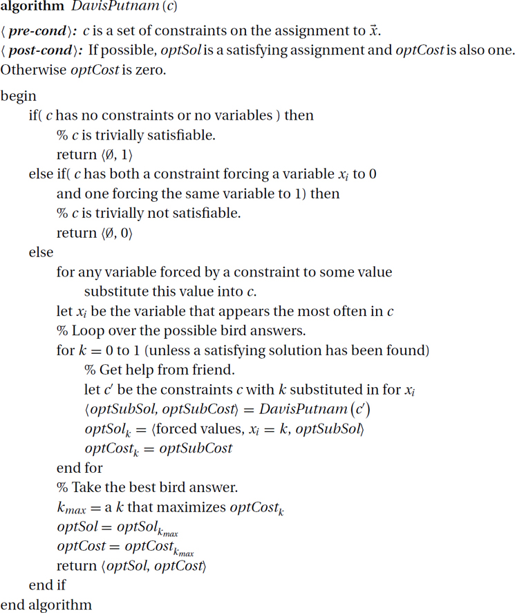
Code:
Running Time: If no pruning is done, then clearly the running time is Ω(2n), as all 2n assignments are tried. Considerable pruning needs to occur to make the algorithm polynomial-time. Certainly in the worst case, the running time is 2Θ(n). In practice, however, the algorithm can be quite fast. For example, suppose that the instance is chosen randomly by choosing m constraints, each of which is the OR of three variables or their negations, e.g., 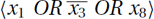 . If few constraints are chosen (say m is less than about 3n), then with very high probability there are many satisfying assignments and the algorithm quickly finds one of these assignments. If a lot of constraints are chosen, (say m is at least n2), then with very high probability there are many conflicting constraints, preventing there from being any satisfying assignments, and the algorithm quickly finds one of these contradictions. On the other hand, if the number of constraints chosen is between these thresholds, then it has been proven that the Davis–Putnam algorithm takes exponential time.
EXERCISE 17.5.1 (See solution in Part Five.) In one version of the game Scrabble, an input instance consists of a set of letters and a board, and the goal is to find a word that returns the most points. A student described the following recursive backtracking algorithm for it. The bird provides the best word out of the list of letters. The friend provides the best place on the board to put the word. Why are these bad questions?
EXERCISE 17.5.2 (See solution in Part Five.) Consider the following Scrabble problem. An instance consists of a set of letters and a dictionary. A solution consists of a permutation of a subset of the given letters. A solution is valid if it is in the dictionary. The value of a solution depends on its placement on the board. The goal is to find a highest-value word that is in the dictionary.
EXERCISE 17.5.3 (See solution in Part Five.) Trace the queens algorithm (Section 17.2.1) on the standard 8-by-8 board. What are the first dozen legal outputs for the algorithm? To save time note that the first two or three queens do not move so fast. Hence, it might be worth it to draw a board with all squares conflicting with these crossed out.
EXERCISE 17.5.4 (See solution in Part Five.) What is the running time of the queens algorithm (Section 17.2.1) for the n-by-n board when there is no pruning? Give reasonable upper and lower bounds on the running time of this algorithm after all the pruning occurs.
EXERCISE 17.5.5 (See solution in Part Five.) An instance may have many optimal solutions with exactly the same cost. The postcondition of the problem allows any one of these to become output. In any recursive backtracking algorithm, which line of code chooses which of these optimal solutions will be selected?
EXERCISE 17.5.6 Suppose you are solving SAT from Section 17.4. Suppose your instance is x AND y, and the little bird tells you to set x to one. What is the instance that you give to your friend? Do the same for instances ¬x AND y, x OR y, and ¬x OR y.
EXERCISE 17.5.7 Independent set: Given a graph, find a largest subset of the nodes for which there are no edges between any pair in the set. Give the bird-and-friend abstraction of a recursive backtracking algorithm for this problem. What do you ask the bird, and what do give your friend?
EXERCISE 17.5.8 Graph 3-coloring (3-COL): Given a graph, determine whether its nodes can be colored with three colors so that two nodes do not have the same color if they have an edge between them. What difficulty arises when attempting to design a recursive backtracking algorithm for it? Redefine the problem so that the input consists of a graph and a partial coloring of the nodes. The new goal is to determine whether there is a coloring of the graph consistent with the partial coloring given. Give the bird-and-friend abstraction of a recursive backtracking algorithm for this problem. What do you ask the bird, and what do give your friend?