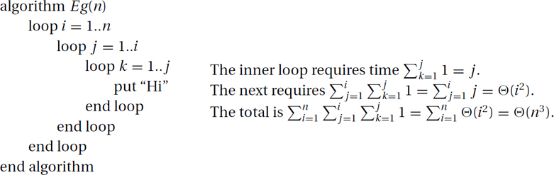
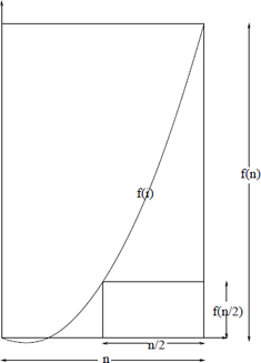
Sums arise often in the study of computer algorithms. For example, if the ith iteration of a loop takes time f(i) and it loops n times, then the total time is f(1) + f(2) + f(3) + · · · + f(n). This we denote as  . It can be approximated by the integral
  , because the first is the area under the stairs of height f(i) and the second under the curve f(x). (In fact, both ∑ (from the Greek letter sigma) and ∫ (from the old long S) are S for sum.) Note that, even though the individual terms are indexed by i (or x), the total is a function of n. The goal now is to approximate for various functions f(i).

Beyond learning the classic techniques for computing  , and
, and  , we do not study how to evaluate sums exactly, but only how to approximate them to within a constant factor. We develop easy rules that most computer scientists use but for some reason are not usually taught, partly because they are not always true. We have formally proven when they are true and when not. We call them collectively the adding-made-easy technique.
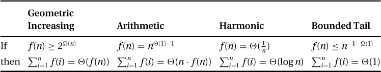
The following table outlines the few easy rules with which you will be able to compute  for functions with the basic form f(n) = Θ(ban · nd · loge n). (We consider more general functions at the end of this section.)
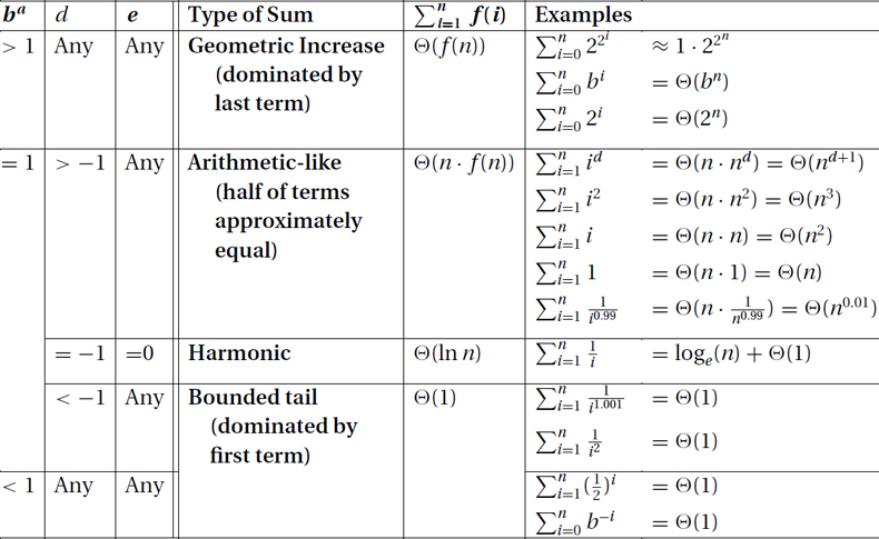
Four Different Classes of Solutions: All of the sums that we will consider have one of four different classes of solutions. The intuition for each is quite straightforward.
Geometrically Increasing: If the terms grow very quickly, the total is dominated by the last and biggest term f(n). Hence, one can approximate the sum by only considering the last term: 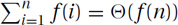 .
.
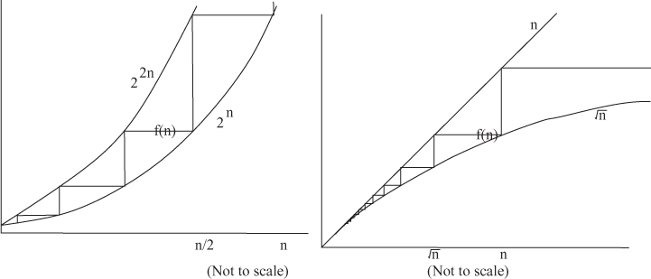
Examples: Consider the classic sum in which each of the n terms is twice the previous, 1 + 2 + 4 + 8 + 16 + · · · + 2n. Either by examining areas within Figure 26.1.a or 26.1.b or using simple induction, one can prove that the total is always one less than twice the biggest term:  . More generally,
 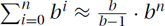 , which can be approximated by Θ(f(n)) = Θ(bn). (Similarly,
 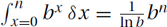 .) The same is true for even fastergrowing functions like
 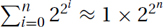 .
.
Figure 26.1: Examples of geometrically increasing, arithmetic-like, and bounded-tail function.
Basic-Form Exponentials: The same technique,  , works for all basic-form exponentials, i.e., for f(n) = Θ(ban · nd · loge n) with ba > 1, we have that
  .
.
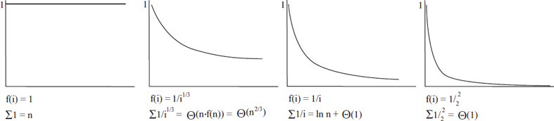
Arithmetic-like: If half of the terms are roughly the same size, then the total is roughly the number of terms times the last term, namely  .
.
Examples:
Constant: Clearly the sum of n ones is n, i.e.,  . This is Θ(n · f(n)).
Linear: The classic example is the sum in which each of the n terms is only one bigger than the previous,  . This can be approximated using Θ(n · f(n)) = Θ(n2). See Figure 26.1.
Polynomials: Both  and more generally
  can be approximated with Θ(n · f(n)) = Θ(n · nd) = Θ(nd+1). (Similarly,
  .)
.)
Above Harmonic:  can be approximated with Θ(n · f(n)) = Θ(n · n−0.999) = Θ(n0.001).
Basic-Form Polynomials: The same technique, , works for all basic-form polynomials, constants, and slowly decreasing functions, i.e., for f(n) = Θ(nd · loge n) with d > 1 we have that  .
.
Bounded Tail: If the terms shrink quickly, the total is dominated by the first and biggest term f(1), which is assumed here to be Θ(1), i.e.,  .
.
Examples: The classic sum here is when each term is half of the previous,  . See Figure 26.1.d and 26.1.e. The total approaches but never reaches 2, so that
  . Similarly,
  and
and  .
.
Basic-Form with Bounded Tail: The same technique, 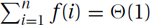 , works for all basic-form polynomially or exponentially decreasing functions, i.e., for f(n) = Θ(ban · nd · loge n) with ba = 1 and d < 1 or with ba < 1.
The Harmonic Sum: The sum  is referred to as the harmonic sum because of its connection to music. It arises surprisingly often and it has an unexpected total:
On the Boundary: The boundary between those sums for which 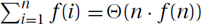 and those for which
 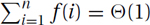 occurs when these approximations meet, i.e., when Θ(n · f(n)) = Θ(1). This occurs at the harmonic function
  . Given that both approximations say the total is
  , it is reasonable to think that this is the answer, but it is not.
The Total: It turns out that the total is within 1 of the natural logarithm, 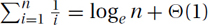 . (Similarly,
 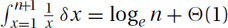 .) See Figure 26.2.
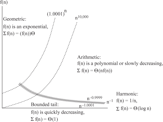
Figure 26.2: Boundaries between geometric, arithmetic, harmonic, and bounded tail.
More Examples:
Geometric Increasing:

Arithmetic (Increasing):

Arithmetic (Decreasing):
Bounded Tail:
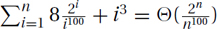
Stranger Examples:
 . Hence,
  .
. .
. , let N = 5n2 + n denote the number of terms. Then
  . Substituting back in for N gives
  .
. .
. , the terms are decreasing fast enough to be bounded by the first term. Here, however, the first term is not Θ(1), but is

 , the first term is f(1) = 2log n−1 · 12 = Θ(n), and the last term is f(log n) = 2log n−logn · (log n)2 = Θ(log2 n). The terms decrease geometrically in i. The total is then Θ(f(1)) = Θ(n).
 .
.EXERCISE 26.1.1 Give the Θ approximation of the following sums. Indicate which rule you use, and show your work.
1. 
2. 
3. 
5. 
6. 
7. 
8. 
9. 
10. 
This section presents a few of the classic techniques for summing and sketches the proof of the adding-made-easy technique.
Simple Geometric Sums:
Theorem: When b > 1,  and when b < 1,
  .
.
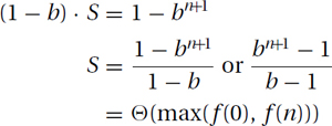
Proof:
Subtracting those two equations gives
Ratio between Terms: To prove that a geometric sum is not more than a constant times the biggest term, we must compare each term f(i) with this biggest term. One way to do this is to first compare each consecutive pairs of terms f(i) and f(i + 1).
Theorem: If for all sufficiently large i, the ratio between terms is bounded away from one, i.e., ∃b > 1, ∃n0, ∀i ≥ n0, f(i + 1)/f(i) ≥ b, then  .
.
Conversely, if ∃b < 1, ∃n0, ∀i ≥ n0,  , then
  .
.
Examples:
Typical: With f(i) = 2i/i, the ratio between consecutive terms is
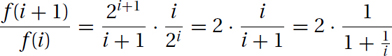
which is at least 1.99 for sufficiently large i. Similarly for any f(n) = Θ(ban · nd · loge n) with ba > 1.
Not Bounded Away: On the other hand, the arithmetic function f(i) = i has a ratio between the terms of  . Though this is always bigger than one, it is not bounded away from one by any constant b > 1.
Proof: If ∀i ≥ n0, f(i + 1)/f(i) ≥ b ≥ 1, then it follows either by unwinding or induction that

See Figure 26.3. This gives that

which we have already proved is Θ(f(n)).
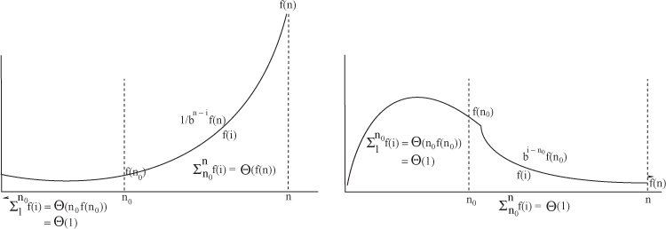
Figure 26.3: In both pictures, the total before n gets sufficiently large is some constant. On the left, the total for large n is bounded by an growing exponential, and on the right by a decreasing exponential.
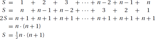
A Simple Arithmetic Sum: We prove as follows that  :
:
Arithmetic Sums: We will now justify the intuition that if half of the terms are roughly the same size, then the total is roughly the number of terms times the last term, namely 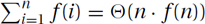 .
.
Theorem: If for sufficiently large n, the function f(n) is nondecreasing, and 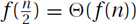 , then .
Typical: The function f(n) = nd for d ≥ 0 is non-decreasing and  . Similarly for f(n) = Θ(nd · loge n). We consider −1 < d < 0 later.
Without the Property: The function f(n) = 2n does not have this property, because  .
.
Proof: Because f(i) is nondecreasing, half of the terms are at least the middle term  , and all of the terms are at most the biggest term f(n). Hence,
  . Because
  , these bounds match, giving
 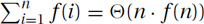 .
.
The Harmonic Sum: The harmonic sum is a famous sum that arises surprisingly often. The total  is within 1 of loge n. However, we will not bound it quite so closely.
Theorem: 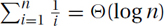 .
.
Proof: One way of approximating the harmonic sum is to break it into log2 n blocks with 2k terms in the kth block, and then to prove that the total for each block is between  and 1:
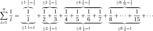
From this, it follows that  .
.
Close to Harmonic: We will now use a similar technique to prove the remaining two cases of the adding-made-easy technique.
Theorem:  is Θ(1) if d′ > 1 and is Θ(n · f(n)) if d′ < 1. (Similarly for f(n) = Θ(nd · loge n) with d < −1 or > −1.)
Proof: As we did with the harmonic sum, we break the sum  into blocks where the kth block has the 2k terms
 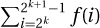 . Because the terms are decreasing, the total for the block is at most F(k) = 2k · f(2k). The total overall is then at most
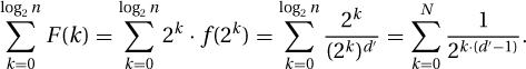
If d′ > 1, then this sum is exponentially decreasing and converges to Θ(1). If d′ < 1, then this sum is exponentially increasing and diverges to  .
.
Functions without the Basic Form: (Warning: This topic may be a little hard.) Until now we have only considered functions with the basic form f(n) = Θ(ban · nd · loge n). We would like to generalize the adding-made-easy technique as follows:
Example: Consider 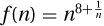 or
or  . They are bounded between
  and
and  for constants d2 ≥ d1 > 0 − 1, and hence for both we have f(n) ∈ nΘ(1)−1. Adding made easy then gives that
 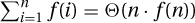 , so that
  and
and  .
.
Counterexample: The goal here is to predict the sum  from the value of the last term f(n). We are unable to do this if the terms oscillate like those created with sines, cosines, floors, and ceilings. Exercise 26.2.4 proves that
  and
and  are counterexamples for the geometric case and that
 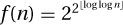 is one for the arithmetic case.
Simple Analytical Functions: We can prove that the adding-made-easy technique works for all functions f(n) that can be expressed with n, real constants, plus, minus, times, divide, exponentiation, and logarithms. Such functions are said to be simple analytical.
Proof Sketch: I will only give a sketch of the proof here. For the geometric case, we must prove that if f(n) is simple analytical and f(n) ≥ 2Ω(n), then ∃b > 1, ∃n0, ∀n ≥ n0, f(n + 1)/f(n) ≥ b. From this, the ratio-between-terms theorem above gives that 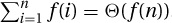 .
.
Because the function is growing exponentially, we know that generally it grows at least as fast as fast as bn for some constant b > 1 and hence f(n + 1)/f(n) ≥ b, or equivalently h(n) = log f(n + 1) − log f(n) − log b > 0 for an infinite number of values for n.
A deep theorem about simple analytical functions is that they cannot oscillate forever and hence can change sign at most a finite number of places. It follows that there must be a last place n0 at which the sign changes. We can conclude that ∀n ≥ n0, h(n) > 0 and hence f(n + 1)/f(n) ≥ b.
The geometrically decreasing case is the same except f(n + 1)/f(n) ≤ b. The arithmetic case is similar except that it proves that if f(n) is simple analytical and f(n) = nΘ(1)−1, then  .
.
EXERCISE 26.2.1 (See solution in Part Five.) Zeno’s classic paradox is that Achilles is traveling 1 km/hr and has 1 km to travel. First he must cover half his distance, then half of his remaining distance, then half of this remaining distance, . . . . He never arrives. By Bryan Magee states, “People have found it terribly disconcerting. There must be a fault in the logic, they have said. But no one has yet been fully successful in demonstrating what it is.” Resolve this ancient paradox by adding up the time required for all steps.
EXERCISE 26.2.2 Prove that if ∃b < 1, ∃n0, ∀i ≥ n0, f(i + 1)/f(i) ≤ b, then  .
.
EXERCISE 26.2.3 A seeming paradox is how one could have a vessel that has finite volume and infinite surface area. This (theoretical) vessel could be filled with a small amount of paint but require an infinite amount of paint to paint. For h ∈ [1, ∞), its cross section at h units from its top is a circle with radius  for some constant c. Integrate (or add up) its cross-sectional circumference to compute its surface area, and integrate (or add up) its cross-sectional area to compute its volume. Give a value for c such that its surface area is infinite and its volume is finite.
EXERCISE 26.2.4 (See solution in Part Five.)
1. For  , prove that f(n) ≥ 2Ω(n)
2. and that  .
.
3. For  , prove that f(n) = nΘ(1)−1
4. and that  .
.
5. Plot  , and prove that it is also a counterexample for the geometric case.
