SO FAR, WE HAVE DEALT WITH THE INHERITANCE of genes in single individuals. The genetic study of a collection of individuals must take into account variations in the population and reasons for those variations. The word “population” simply refers to large numbers of individuals able to breed: for example, human populations. The genetics of whole populations is useful for predicting the chances of genetic diseases occurring in large groups of individuals. It is also the basis for understanding differences in the frequency of traits or diseases in different ethnic groups.
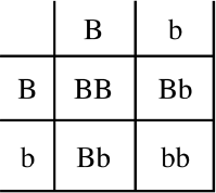
In chapter 3 we saw that the laws of Mendelian inheritance apply to people too. At first, many scientists did not easily accept this idea. The first case of a dominant trait discovered in humans, in 1903, was brachydactyly. This condition is characterized by shortened or fused fingers and toes. Based on the low frequency of this condition in the population at large, some scientists stated that Mendelian genetics did not apply to people. One wrote, “If Mendelian Laws of Genetics apply to people, and brachydactyly is a dominant trait, why don’t 3 out of 4 people have brachydactyly?” (Udny Yule, cited in G. H. Hardy, “Mendelian Proportions in a Mixed Population,” Science n.s. 28 (1908): 49–50). You see, this scientist drew a Punnett square with two heterozygotes for brachydactyly as parents and saw that 75 percent of the offspring must have the brachydactyly trait (figure 10.1). Since 75 percent of the population doesn’t have brachydactyly, he claimed that Mendelian laws of genetics do not apply to people! Can you see what is wrong with his logic? The prediction of 75 percent brachydactyly only applies if two heterozygotes for brachydactyly have children, in which case the prediction is absolutely correct. Since most people do not have brachydactyly, most parents are normal and do not expect to have any brachydactyly children. The flaw in the logic was pointed out by an English mathematician, Godfrey H. Hardy, and by Wilhelm Weinberg, a German physician. Both provided the correct explanation as to why a dominant trait does not appear three times more frequently than a recessive trait in a population. Thus, predictions regarding genotype frequencies in populations is called the Hardy-Weinberg law. This law is useful for calculating approximate frequencies of genes and genotypes in populations.

Figure 10.1 A Punnett Square Used to Predict the Offspring of Heterozygous Brachydactyly Parents. With these parents we would expect 75 percent brachydactyly children and 25 percent normal since brachydactyly is a dominant trait. However, this prediction is true only if both parents are heterozygous for brachydactyly.
The Hardy-Weinberg law is a direct extension of how genes are passed down from parents to offspring on an individual basis to the same process for a whole population. Because of this, we will again use a Punnett square. Recall that in setting up the Punnett square, we put the genotype of the gametes from one parent on top and the other parent on one side. Then, we carry down the gene from one parent and carry across the gene from the other parent to determine the genotypes and their proportions in the next generation. When we want to extend this Punnett square analysis to a whole population, we must include the genes from all parents in this population. When we include all, rather than individual, parents, the proportions of different genes present in the population are represented.
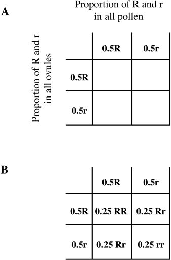
Let’s take a hypothetical example of a field of flowers. Let’s say we planted a field of pink four-o’clock flowers. Recall from chapter 2 that four-o’clock flower color is a case of incomplete dominance in which heterozygotes Rr are pink, homozygotes RR are red, and homozygotes rr are white. So, if the whole field has pink flowers we know that all the plants have the genotype Rr. If these flowers were to pollinate each other, we can predict what the proportions of resulting offspring will be. Remember that Rr parents will all generate equal numbers of Rand r-carrying gametes. This can be represented in a Punnett square as 50 percent, or 0.5 R and 0.5 r, for all parents (figure 10.2). Then, we multiply the numbers for each of the genotypes to get 0.25, or 25 percent, for each of the four categories of offspring. The interpretation of this Punnett square is that in the next generation in that field, there will be approximately 25 percent RR, or red, 50 percent Rr, or pink, and 25 percent rr, or white flowers. This result would be expected if each flower had equal chances of pollinating and being pollinated, each resulting fertilized flower set its seeds, and all the seeds grew into new plants.
Suppose now we come back the following year to look at this field of flowers that, now, has red, pink, and white flowers in a 1:2:1 (25 percent, 50 percent, and 25 percent) ratio. What frequency of red, pink, and white flowers do we expect to see next year? First of all, what is the frequency, or the proportion, of R and r genes in the flowers this year? We can calculate it since we know the proportion of the three genotypes:
| For 0.25 RR |
0.25 R |
| For 0.5 Rr |
since half of 0.5 is 0.25, we get 0.25 R and 0.25 r |
| For 0.25 rr |
0.25 r |
So, in total, there are 0.5 R genes and 0.5 r genes, which is what we started with when we had all pink flowers in our field! Let’s now calculate what proportion of different colored flowers we expect the following year. As before, we need to calculate the percentage of R and r genes in the population. In this case, we observe 25 percent RR (or 0.25 R), 50 percent Rr (0.25 R + 0.25 r) and 25 percent rr (or 0.25 r). The ratio of R versus r is again 0.5 to 0.5, the same as what we found in the previous generation! So, in future generations we expect the same result, that starting with a field of 25 percent red, 50 percent pink and 25 percent white flowers, we again will get 25 percent red, 50 percent pink and 25 percent white flowers. The fact that the proportion of genes and genotypes did not change from one generation to the next demonstrates that gene frequency, or the proportion of different forms of the gene, and genotype frequency both stay the same. This is what the Hardy-Weinberg law states: in populations, gene and genotype frequencies do not change over successive generations. We will see next, however, that certain conditions must be roughly true for this law to be applicable.

Figure 10.2 Using a Punnett Square to Calculate Genotype Frequencies. A. The gametes from all male parents (pollen) are shown at the top and gametes from all female parents (ovules) are shown at the side with 0.5 gene frequency. B. We multiply the gene frequencies to calculate the genotype frequencies. This example shows that all four genotypes occur at 0.25 frequency, or 25 percent each.
So, what are the conditions important in keeping the gene and genotype frequencies constant? One important assumption is that we expect all the flowers to contribute equally to the next generation. For example, if insect pollinators favored the red over the pink and did not visit white flowers at all, the r form of the gene would be underrepresented in the next generation. This is one type of “selection,” and such selection would alter the proportion of the genes that are passed down to the next generation. Also, there should not exist a situation in which different insects only visit one color of flowers. For example, let us imagine that one type of insects only visited red flowers, another type only pink, and another type visited just the white flowers. This is an example of nonrandom mating. In this case, the red flowers would produce only more red flowers, white flowers would only give rise to white flowers, and the pink flowers would give rise to red, white, and pink. Thus, we would get fewer pink flowers than what the Hardy-Weinberg law would predict.
It is also necessary that the wind or the insect pollinators do not bring in pollen from other fields. For example, if the adjoining farm grew all red flowers, because they fetched a better price, and pollen from that field drifted into ours, more of the R gene than predicted would be represented in the next generation. This effect is called “migration,” that is, migration of genes from someplace else. The numbers predicted by the Hardy-Weinberg law would also be distorted if pollen from our field were blown somewhere else, that is, migrated away, and became unable to pollinate the flowers in our field. We also hope, and reasonably so, that the mutation rate would be too low to change the frequency of the two forms of the gene. Finally, for the prediction to hold, we must have a reasonable number of flowers in the field. That is, if we had a tiny field with only a few flowers, random chance could alter the proportion of genes that gets passed down to the next generation.
Can we use these predictive tools with humans? Are the conditions of no selection, no migration, random mating, no mutation, and large population size applicable to humans? In fact, for most traits of interest, these conditions do not strictly hold true. Indeed, in the case of genetic diseases, there is clearly selection against individuals with the disease trait. For example, males very sick with hemophilia may not survive long enough to have children. Also, certainly, we would like to think that humans do not mate randomly! And we know further, especially in the United States, that people move quite easily from place to place and even across huge oceans and continents. So, does this mean that the Hardy-Weinberg law demonstrated with the four-o’clock flower is not applicable to humans? No, in many cases, it actually is applicable. This law can be thought of as a “back of the envelope” calculation that gives us an approximate proportion of genes and genotypes in a human population. As long as we keep this in mind, the Hardy-Weinberg law can be a very useful tool.
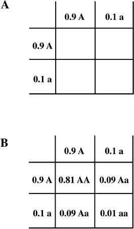
Now that we have learned how to use the Punnett square to estimate genotype frequencies in successive generations at the level of a whole population, let us study a general example. Rather than considering 50 percent each of the two forms of the gene as in the four-o’clock plant example, let us try a calculation with 10 percent, or 0.1, of the a form and 90 percent, or 0.9, of the A form (figure 10.3). Multiplying through, we expect among the offspring 0.01, or 1 percent, aa; 0.09 + 0.09 = 0.18, or 18 percent Aa; and 81 percent AA. If all the conditions mentioned above hold, we expect the proportions of the genes and genotypes to remain the same in the following generations. Let us see if this is true. What are the proportions of a and A in the second generation with 1 percent aa, 18 percent Aa, and 81 percent AA?
| 1 percent aa gives |
0.01 a |
| 18 percent Aa gives half of 0.18 |
|
| each for A and a, or |
0.09 a and 0.09 A |
| 81 percent AA gives |
0.81 A |
This gives a total of 0.01 a + 0.09 a = 0.10 a, and 0.09 A + 0.81 A = 0.90 A.
Figure 10.3 Using the Punnett Square to Calculate the Proportion of Genotypes in the Next Generation Beginning with Gene Frequencies of 10 Percent a and 90 Percent A. A. The gene frequency filled in for all reproductive males and females. B. The whole Punnett square filled in with genotype frequencies.
So indeed, the gene frequency remains constant if we allow all the genotypes to contribute equally to the next generation and do not remove or add genes from another population. And if gene frequencies are constant, we expect the genotype frequencies to stay constant, provided the conditions of no selection, random mating, no migration, no mutation and large population size are generally true. But surely, we did not learn the Hardy-Weinberg law just to talk about hypothetical example of field of flowers! You’ll see next that this law is also useful for predicting genotype frequencies for human genetic diseases.
Now, let’s see if we can use the Hardy-Weinberg law to illustrate the case of a human recessive disease. As mentioned already, we do expect selection against disease traits, but we can still use the Hardy-Weinberg law to make some predictions. But first, in humans, unlike the examples with flowers, we often do not know the frequency of a recessive gene in the population. The disease trait is phenotypically expressed for a recessive trait only when an individual is homozygous recessive. Thus, the information we can gather is the number of affected individuals in the population, that is, the proportion of homozygous recessive individuals in the population under study. How can we use this information?
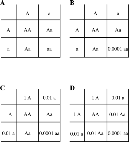
Let’s again apply the Punnett square (figure 10.4), using as an example the human recessive disease PKU that we learned about in chapter 3. We can fill in the genes and genotypes (figure 10.4.A). Now, we know from medical records that roughly 1 in 10,000 U.S. Caucasians suffer from PKU. This is 0.0001 in decimals, or in scientific notation, 10-4. This number represents the proportion of homozygous recessive individuals so we’ll associate that number with the genotype aa (figure 10.4.B). The proportion of the a gene in the population is thus the square root of the proportion of aa, since the number of a multiplied by itself gives aa. The square root of 0.0001, or 10-4, is 10-2, or 0.01, or 1 percent. The frequency of the normal A gene is thus 1 − 0.01 = 0.99, or 100 percent − 1 percent = 99 percent. We now have the full information necessary to fill out this Punnett square for estimating the frequency of the PKU gene in the population (figure 10.4.D). Therefore, from only knowing approximately how many individuals suffer from PKU, we can estimate the frequency of the PKU gene in the U.S. Caucasian population. This frequency is 1 percent.
An even more useful piece of information we can estimate is the proportion of carrier individuals in the population. As you see from the Punnett square (figure 10.4.D), this proportion is twice 10-2, or 0.02, or, to put it another way, 2 out of 100 individuals (2 percent) are carriers. This may seem to be a surprisingly large number for a disease with a frequency of only 1 out of 10,000 people, but it is correct. This is one very useful aspect of the Hardy-Weinberg law of population genetics: it allows us to calculate the carrier frequency, something that cannot easily be determined in any other way.
Figure 10.4 A Punnett Square Used to Calculate the Frequency of Recessive Disease Genes in a Population. A. Punnett square with just the genes showing. B. As A, with the frequency of aa individuals shown. C. As B, with the calculated frequency of the a gene calculated. D. Complete Punnett square. To simplify, we write “1 A” rather than “.99 A.”
The PKU example also illustrates why it is valid to use this law even when the trait is clearly selected against. (PKU individuals, until newborn PKU testing became widespread, were mentally retarded and unlikely to reproduce). Let us calculate what percentage of the PKU gene in the population is carried by affected homozygous individuals, as compared to the percentage carried by phenotypically normal heterozygous individuals. We know at the outset that there is a proportion of 1 in 10,000, or 0.0001, homozygous recessive PKU individuals, and we calculated the percentage of carrier individuals as 0.02. So the proportion of PKU genes carried by homozygous individuals who have 2 copies of the PKU gene is 2 × 0.0001 = 0.0002, and that carried by heterozygous individuals is 0.02. The total is 0.0202. Thus the proportion of the gene carried by homozygous recessive individuals is 0.0002 divided by 0.0202, or ~1 percent. This means that PKU individuals carry less than 1 percent of the total PKU genes in the population, while greater than 99 percent of the PKU gene in the population is carried by phenotypically normal heterozygous individuals. So, even if none of the PKU individuals passed their PKU genes to the next generation, 99 percent of the PKU genes will still be passed onto the next generation by heterozygous carrier parents.
You may have noticed that we stated the frequency of PKU specifically for U.S. Caucasians. Why did we do this? Is the frequency different among different ethnic groups? Depending upon the evolutionary and genetic history of different ethnic groups, frequencies of different genes are different. For example, in the case of PKU, as we saw, the frequency among U.S. Caucasians is approximately 1 in 10,000. However, the frequency of PKU among African Americans is lower, only around 1 in 50,000. Among ethnic Japanese, it is even lower and stands at approximately 1 in 110,000. On the other hand, sickle-cell anemia is much more prevalent among African Americans, at 1 in 400, while the prevalence among the general population is around 1 in 2,500. We will discuss the causes for these differences in the next chapter.
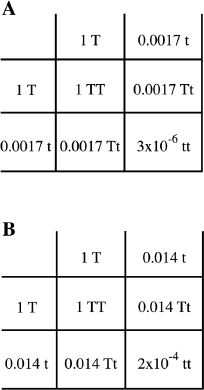
One extreme example of differences in the frequency of a disease among populations is Tay-Sachs disease. This is a non-sex-linked recessive disease that affects the nervous system. It has no cure or treatment, and affected babies die by the age of two or three. Because it is a recessive disease, two phenotypically normal parents, if they are heterozygous for the trait, have a 25 percent chance of having an affected baby (recall chapters 2 and 3). Fortunately, this disease is quite rare in the general population, with a frequency of about 1 in 360,000 or about 3 × 10⁻⁶. We can use the Punnett square to estimate the frequency of carrier individuals in the general population (figure 10.5.A). The square root of 3 × 10⁻⁶ is approximately 0.0017, and thus the carrier frequency is approximately 2 × 0.0017 or about 0.0035, or in other words a little more than 3 out of 1,000 people in the general population are carriers. Thus, the chances are quite small that two carrier individuals will marry and have children. However, it turns out that the frequency of this trait is unusually high among Ashkenazi Jews of Eastern European origin. In that population, Tay-Sachs is found in roughly 1 out of 4,800 individuals or approximately 2 × 10⁻⁴. Also, the values for the general population hold true for the population of New York City, and the values for Ashkenazi Jews of Eastern European origin hold true for members of this community who live in New York City. Clearly, there is not random mating among these groups in NYC, and these groups are reproductively separate. We again use the Punnett square to calculate the frequency of carrier individuals (Figure 10.5.B). The square root of 2 × 10⁻⁴ is approximately 0.014, the gene frequency, and the carrier frequency is twice that, or 0.028, or roughly 1 in a 30, or approximately 3 percent, are carriers. This is a much higher carrier frequency than for the general population. The higher frequency predicts a greatly increased chance that two heterozygous individuals from this subgroup in New York City will marry and have children. Tay-Sachs is also unusually high among French Canadians and the Cajuns of Louisiana. For this reason, testing is now available for individuals from these groups to determine if they are carriers.
How is the knowledge about the frequency of different genes and genotypes in the population useful? As mentioned already, all fifty states test for PKU among their newborns. The accuracy of most of the newborn testing is better than 99.9 percent. Thus, these tests are very accurate but not perfect. Because the tests are accurate, we expect that any baby born with the disease will be detected. However, there is a 0.1 percent chance that even if a baby does not have the disease it will test positive. That is, there is a 0.1 percent chance of false positive. So, let’s see the consequences of this false positive result.
Figure 10.6 shows how many babies will test truly positive compared to the false positives. First, we begin by choosing the total number of individuals tested. In Figure 10.6.A we chose 10,000, since the frequency of PKU among U.S. Caucasians is 1 in 10,000. Then we make a row for those that test positive and a row for those that test negative. After that, we make a column for the number of individuals we expect to be affected and for those that are not affected. Only one affected baby is expected, and that baby will test positive. Under the designation “normal,” we use the information we have regarding false positives to fill in the “test positive” category. The false positive rate is 0.1 percent; 0.1 percent of 10,000 is 10. Thus ten normal babies will test positive! The remainder of the babies will test negative. Now we can calculate the total for those that test positive. Of the 11 that test positive, only 1 is expected to actually have PKU. Any baby that tests positive for any disease is automatically tested again because of these unavoidable false positives. It is highly unlikely that testing the same baby will yield a false positive twice in a row. It is only after a baby tests positive twice that doctors are contacted to check the diagnosis and begin treatment.

Figure 10.5 Using the Punnett Square to Calculate the Proportion of Tay-Sachs Carriers. A. Among the general population. B. Among Ashkenazi Jews of Eastern European origin.
Now, let’s do the same analysis, using this time the PKU rate among ethnic Japanese. In this population, PKU is found at the much lower rate of 1 in 110,000. We fill in the same table as before in figure 10.6.B, but we choose 110,000 as the total population, since now there is only 1 case of PKU in 110,000 births. The number of affected babies is just one, and that one will be detected as positive. However, although the accuracy of the test does not change, the false positive rate of 0.1 percent now applies to a much larger population, so the actual number of false positives is 110. So now out of a 111 that test positive, only 1 baby actually has PKU! This conclusion strongly reinforces the necessity of conducting more than a single test to determine which babies are truly PKU positive.
Figure 10.6 Calculating the Number of False Positives for PKU. A. In the case of the U.S. Caucasian population. B. In the case of the Japanese population.
The actual number of disease cases relative to the number of false positives is an important consideration when deciding whether to screen the general population. Another example of this is maple syrup (or fenugreek) urine disease. This is a metabolic genetic disease that can be easily treated with vitamins and dietary control. This disease is quite rare in the general population, and the estimated frequency is about 1 in 300,000. In several years of testing newborns in Iowa, all babies that tested positive turned out to be false positives. Therefore, testing for this disease was discontinued in Iowa in 1995. There are populations that have unusually high rates of this disease, for whom testing is advised. For example, a Mennonite community in eastern Pennsylvania has a rate of 1 in less than 200! We discuss possible reasons for such differences in disease frequency in the next chapter.

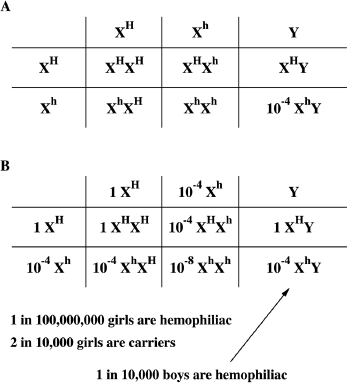
Figure 10.7 Punnett Squares Used to Calculate the Frequency of a Sex-Linked Trait in a Population. A. Punnett square representing the males at the top and the females on the side. The males are represented by two X chromosomes for the frequency of the normal and disease gene on the X chromosome and by their Y chromosome. The 1 in 10,000 frequency for hemophilia A among males of is shown for XhY. B. Completed Punnett square with the hemophilia gene frequencies.
We saw in chapters 2 and 3 that we can use the Punnett square to predict the proportion of genotypes in offspring for sex-linked traits (figure 10.7). Similarly, we can use a modified Punnett square to calculate the genotype frequency for sex-linked traits for a population. When we deal with sex-linked traits, the Punnett square has the sex chromosomes represented for the mother by X and X, and for the father by X and Y. The trait we will be discussing is hemophilia, an X-linked trait. Thus, there exists in the population a fraction of X chromosomes with the normal gene, XH, and another fraction with the hemophilia gene, Xh. Although each individual male in the population has only one X chromosome, to represent all the males in the population, we need to represent males with both XH and Xh. In order to represent the frequency of the two different forms of the gene on the X chromosome, males are represented by two X chromosomes and a Y chromosome. Now we can insert the information that we have, that approximately 1 in 10,000 males, or 0.0001, or 10-4, in the population has hemophilia A (figure 10.7.A). Since this number is the result of multiplying the frequency of Y (which is 1, or 100, percent among males) with the frequency of Xh, the proportion of hemophilia among males is the same as the proportion of the hemophilia gene on the X chromosomes in the whole population. So, we can indicate 0.0001 or 10-4 as both the frequencies of Xh among males (top) and among females (side). Again, because this is such a small number, for ease of calculation we use 1 for the frequency of XH instead of (1 – 10-4). Now we can finish calculating the genotype frequency among the female offspring. Since the genotype frequency in females is calculated by multiplying the frequency of Xh by itself, the frequency of hemophiliac girls is estimated to be about 0.00000001, or 10-8, or 1 in 100 million, and the frequency of carrier girls is about 2 in 10,000. So, just as we saw in chapter 3, we expect and observe that men have a much higher frequency of X-linked diseases than women.
In this chapter, we extend the rules of Mendelian genetics from individuals to whole populations. We can predict the gene and genotype frequency in a population using a modified Punnett square. The rules of Mendelian genetics extend to populations of people and allow us to predict genotype frequencies by using the Hardy-Weinberg law. The Hardy-Weinberg law shows that in a large population, if all the genes have equal probability of being passed down to the next generation, gene and genotype frequencies remain constant. Understanding how genes are passed down in populations allows us to estimate the proportion of carriers of recessive genetic diseases. There exist cases of very different frequencies of genetic diseases among subgroups of the population. The existence of different gene frequencies suggests nonrandom mating among these groups. Knowing the predicted frequency of diseases allows us to decide whether there should be population screening for genetic diseases.
