3
Clathrate Nano-Cages
Clathrates or gas hydrates were discovered by D. Humphrey in 1810. After being virtually ignored for a long time, studies on the thermodynamic conditions of their formation gained importance in the 1930s when gas transport via pipelines had become problematic at low temperatures due to the formation of blockages that slowed down or prevented the flow of these gases.
Nowadays, from a point of view of planetology, it is accepted that clathrates could exist in many solar system bodies: giant planets, on the surface and inside Titan, satellite of Saturn, comet nuclei or even the polar regions of Mars.
Indeed, several atomic and molecular species, which have been observed in the atmosphere of this planet: carbon dioxide (CO2), the major constituent, methane (CH4), noble gases and other species, could have been stored in the form of clathrates in the Martian subsoil [CHA 07, THO 09, MOU 12].
On our planet Earth, clathrates (carbon dioxide, methane, etc.) are present in certain marine sediments, in the permafrost (permanently frozen soil) and in lakes under Antarctic ice layers. Methane clathrates could be a source of significant climate change if this methane were to be released (its heating power is 20 times more powerful than that of carbon dioxide)!
Observations in the cold regions of interstellar media revealed the presence of ice grains containing atoms, radicals and simple molecules such as H2, CO, CO2, CH4, HCN, NH3, CH3OH, H2CO, and also more complex molecules such as polycyclic aromatic hydrocarbons (PAH) [DRA 88, MAT 89].
Very recently, the detection of molecular oxygen O2 in the gas cloud surrounding the comet 67P/Tchourioumov–Guerassimenko, by the spectrometer Rosina on board the European probe Rosetta, has stunned the scientific community interested in comets. Indeed, no scientist had previously tried to detect dioxygen as its presence seemed unlikely. Abundance measurements around the comet have shown that O2 is the third most abundant species after H2O and CO2 [BIE 15].
3.1. Introduction
Determining the presence and evolution of molecular species and their physicochemical environment in astrophysical media makes high-resolution infrared spectroscopy a powerful investigative tool that would provide a great deal of information on how these molecules behave in their environments.
In this chapter, we describe the theoretical models developed to analyze the absorption spectra of a triatomic molecule trapped in a clathrate nano-cage at very low temperatures. The Lakhlifi–Dahoo extended inclusion model allows the determination of the trapping site (cage structure type), position and movements of the molecule in its site. Frequency shifts due to the solid environment can be interpreted using an atom–atom potential model to describe the interaction between the clathrate matrix and the trapped molecule. Moreover, this inclusion model makes it possible to determine the IR spectra and the couplings with the atoms or molecules forming the nano-cage.
The study of these different aspects calls for a detailed modeling, not only of the clathrate structure at the molecular scale, but also of the spectroscopic response of host molecules. Indeed, spectroscopy is a non-destructive investigation method and the comparison of experimental results with those from theoretical models will make it possible to establish the validity of the models used to represent the host molecule–water molecule interactions inside clathrates.
Unlike an ordinary ice crystal that is formed from pure water in a hexagonal structure, clathrate crystals are formed, under particular temperature and pressure conditions, from water containing dissolved gaseous species. In these crystals, water molecules are organized around a small “host” or “trapped” gas atom or molecule, and form a compact assembly of nano-cages, according to well-identified structures.
In such structures, stability is ensured by hydrogen bonds that are established between the water molecules, and the van der Waals bonds between the trapped species and the surrounding water molecules, at a minimum filling rate. In addition, the type of clathrate structure formed is determined by the size of the host atom or molecule. There are several types of clathrate hydrate structures. The three types of structures that the great majority of natural clathrates have are I, II and H structures (denoted sI, sII and sH).
In the extended Lakhlifi–Dahoo substitution model, the effective charges calculated by quantum chemistry methods are used to determine the electric field of the environment in which the molecule evolves within a nano-cage. In this case, the effective charges are placed on each atom of the trapped molecule and the molecules constituting the nano-cage structure.
3.2. Clathrate structures
All clathrate structures consist of unit cells (or elementary cells) containing cages of different sizes in the form of polyhedra (Figure 3.1). The number of cages and their organization are different according to their size and the structure to which they belong [SLO 08].

Figure 3.1. Unit cells of clathrate crystals: (a) structure sI, (b) structure sII and (c) structure sH. For a color version of this figure, see www.iste.co.uk/dahoo/infrared2.zip
In the structures sI, sII and sH, we find the following polyhedra:
- – the pentagonal dodecahedron 512 formed with 12 pentagons and is known as a “small cage”. It contains 20 water molecules, and is found in the structures sI, sII and sH;
- – the tetradecahedron 51262 formed with 12 pentagons and two hexagons facing each other and is each surrounded by six pentagons. This polyhedron is known as a “large cage” and contains 24 water molecules. It is only found in the structure sI;
- – the hexadecahedron 51264 formed from 12 pentagons and four hexagons whose position is such that their center is at the top of a tetrahedron and each one is surrounded by six pentagons. This polyhedral is known as a “large cage” and contains 28 water molecules. It is found only in the structure sII;
- – the irregular dodecahedron 435663 formed of three squares, six pentagons and three hexagons. This polyhedron is a “medium cage” and contains 20 water molecules. It is only found in the structure sH;
- – the icosahedron 51268 formed of 12 pentagons and eight hexagons. It is known as “large cage” and contains 36 water molecules. It is only found in the structure sH.
Each structure crystallizes according to a crystallographic system whose unit cell contains a certain number of cages and water molecules:
- – the unit cell of the sI structure is cubic, composed of two small cages and six large cages and contains 46 water molecules. Its cell parameter is a = 12.00 Å;
- – the unit cell of the sII structure is face-centered cubic, composed of 16 small cages and eight large cages and contains 136 water molecules. Its cell parameter is a = 17.30 Å.
These two structures can be stabilized by small atoms or molecules: rare gas atoms, O2, CO2, H2S, HCN, NH3, CH4, C3H8, etc. Table 3.1 presents some information concerning these two structures, and in Figure 3.2, we show the three types of cages forming these structures.
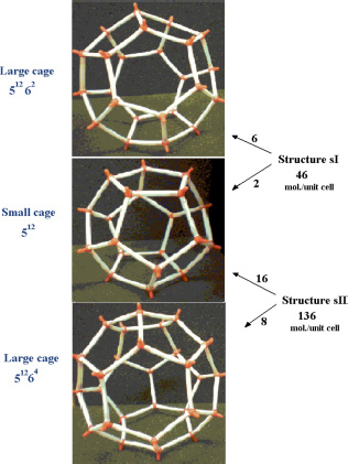
Figure 3.2. Small and large cages forming sI and sII structures, and the number of water molecules per unit cell. For a color version of this figure, see www.iste.co.uk/dahoo/infrared2.zip
Table 3.1. Some data on sI and sII clathrates [SLO 08]
| Clathrate type | Structure sI | Structure sII | ||
| Unit cell | Cubic | Face-centered cubic | ||
| Cell parameter a (Å) | 12.00 | 17.30 | ||
| Number of H2O per unit cell | 46 | 136 | ||
| Cage size | Small 512 |
Large 51262 |
Small 512 |
Large 51264 |
| Number of cages per unit cell | 2 | 6 | 16 | 8 |
| Mean radius (Å) | 3.95 | 4.33 | 3.91 | 4.73 |
- – the unit cell of the structure sH is hexagonal, composed of three small cages 512 with an average radius of 3.94 Å, two medium cages 435663 with an average radius of 4.04 Å and one large cage 51268 with an average radius of 5.79 Å, and contains 34 water molecules.
To be stabilized, this structure requires the presence of small molecules and larger molecules, which is not the case of the molecules that interest us. Hence, we will not consider this structure in the rest of this chapter.
3.3. Inclusion model of a triatomic molecule in a clathrate nano-cage
The construction of a realistic theoretical model allowing the quantitative interpretation of the spectroscopic and thermodynamic phenomena of a molecule in a nano-cage requires a good knowledge of the interaction potential energy between this molecule and the atoms or molecules constituting the nano-cage. This energy must, however, have an analytical form showing a clear dependence of the degrees of freedom of the active molecule and its partners, that is, their position, their orientation and their internal vibrations.
This interaction energy is generally considered as a result of pairwise (binary) interactions between the trapped molecule and each atom or molecule of the nano-cage.
3.3.1. Inclusion model
Consider a triatomic molecule, initially assumed to be rigid, trapped in a small or large cage of clathrate structure sI or sII, also assumed to be rigid. The positions of the hydrogen and oxygen atoms are defined by their coordinates in a fixed reference frame linked to the crystalline clathrate lattice, whereas those of the atoms constituting the trapped molecule are defined by their coordinates in the mobile frame linked to the equilibrium configuration of the molecule. Figure 3.3 shows, for example, the model trapping of a carbon dioxide CO2 molecule in a small cage 512 of the clathrate structure sI and the fixed reference frame  linked to this structure.
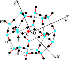
Figure 3.3. Trapping of a triatomic molecule in a small cage of clathrate structure sI.  , is the fixed reference frame (laboratory frame) linked to the clathrate matrix. For a color version of this figure, see www.iste.co.uk/dahoo/infrared2.zip
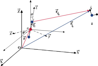
Figure 3.4. Geometric characteristics of a CO2–H2O couple. The position of the center of mass G and the orientation of the molecule are defined relative to the fixed reference frame linked to the clathrate matrix. For a color version of this figure, see www.iste.co.uk/dahoo/infrared2.zip
Most of the time, the environmental effects of each species are taken into account using actual parameters of the binary potential energy. Figure 3.4 shows the geometric characteristics of a “trapped molecule–water molecule of the matrix” couple and the positions of the internal sites of the trapped molecule relative to its reference frame  as well as its external, orientational and translational degrees of freedom, relative to the fixed reference frame .
3.3.2. Interaction potential energy
This pairwise potential energy is the sum of long-range contributions of electrostatic, inductive and dispersive natures (van der Waals interactions) and short-range repulsive contributions describing, on the one hand, the overlapping of electron orbitals of the two species, and on the other hand, possible charges transfer phenomena. The analytical expressions of the different contributions were presented in Chapter 4 of Volume 1 of this series [DAH 17].
In the case of a molecule trapped in a rigid clathrate nano-cage, the dispersion–repulsion contribution is modeled by the sum of Lennard-Jones 6–12 potential energies. Moreover, since the distance between the trapped molecule and the water molecules is small (approximately the size of a molecule), these molecules also interact through their electric charge distributions, which can be found in each molecule, on its atoms or on other sites. The interaction potential energy  between the trapped triatomic molecule and the water molecules in the clathrate crystal “structure-cage s-c” (with s = sI or sII and c = s for small or l for large) is given by:
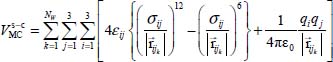
In this expression, NW is the number of water molecules in the clathrate matrix,  is the distance vector between the site i, with an electric charge qi, of the trapped molecule, on the one hand, and the site j, with an electric charge qj, of molecule k in the clathrate matrix, on the other hand; in contrast, εij and σij are site-site Lennard-Jones potential parameters determined by the following Lorentz–Berthelot combination rules:

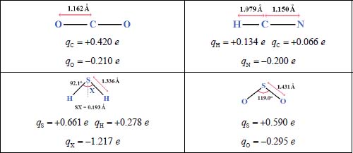
where (εii, σii) are the Lennard-Jones parameters of a pair of identical atoms i−i in the gas phase. These parameters are determined using quantum chemistry numerical techniques (semi-empirical, ab initio, etc.), and their value for the atoms present in this study is given in Table 3.2 [LAK 84, WAL 95, KET 11]. The distribution of the effective electric charges in clathrate water molecules is: qH = +0.4238 e and qO = −0.8476 e [ALA 09], those concerning the trapped molecules will be presented later on.
Table 3.2. Lennard-Jones parameters. Energy conversion factor: 1 meV = 8.06554 cm−1
| i – i pair | H – H | O – O | C – C | N – N | S – S |
| εii (meV) | 0.7402 | 4.9470 | 3.6947 | 3.2137 | 6.3591 |
| σii (Å) | 2.810 | 3.030 | 3.210 | 3.310 | 3.390 |
Moreover, the coordinates of each hydrogen atom and each oxygen atom of the matrix are listed in a data file for each type of structure. We will consider the following for numerical calculations:
- – a 4 × 4 × 4 dimension matrix formed of 64 unit cells (i.e. 2,944 water molecules), for the structure sI;
- – a 3 × 3 × 3 dimension matrix formed of 27 unit cells (i.e. 3,672 water molecules), for the structure sII.
These matrices are large enough to ensure a good convergence of the “trapped molecule–clathrate matrix” interaction energies.
In order to study the movements of the molecule trapped in its cage, the dependence of the interaction energy  in terms of the internal (vibration) and external (translation and orientation) degrees of freedom of the molecule must be clearly determined. Thus, the distance vector
  of expression [3.1] can be written as:

where  and
and  are respectively the position vector of the center of mass G of the trapped molecule and the position vector of atom j of molecule k of the clathrate matrix with respect to the fixed reference frame
  ; and
; and  is the position vector of atom i of the trapped molecule with respect to its reference frame
  . The latter is then developed as a Taylor series with respect to the normal vibrational coordinates:
and expressed relative to the fixed reference frame using the unitary rotational matrix transformation M(φ, θ, χ) (Appendix 2.7.1, Chapter 2), which makes it possible to accurately determine the angular coordinates  of the molecule (
 for a linear molecule) in its site.
3.4. Thermodynamic model of clathrates
In order to study the evolution and the environmental impact of the chemical composition of the atmosphere of a planetary body, planetologists need to determine the relative abundance of potentially trapped chemical species in clathrate cages; that is, the occupation fractions of these species under the thermodynamic conditions of temperature and pressure where the clathrates are formed.
From a theoretical point of view, the thermodynamics of clathrate formation or dissociation is frequently based on the van der Waals and Platteeuw model [VAN 59], a three-dimensional generalization of the Langmuir theory [LAN 16] on the adsorption of a gas onto a surface. This model is based on the following assumptions:
- 1) The contribution of the matrix water molecules to the free energy is independent of the occupation mode in the cages. This particularly implies that the trapped molecules do not deform the cages.
- 2) The trapped molecules are supposed to be rigid and are confined in their supposedly rigid cage, at a rate of one molecule per cage.
- 3) The mutual interactions between trapped molecules are negligible, in other words, the partition function of the motions of a molecule trapped in a cage is independent of the other trapped molecules.
- 4) The quantum effects are negligible.
3.4.1. Occupation fractions and Langmuir constants
The relative abundances of gaseous species trapped in a clathrate can be calculated using the laws of classical statistical mechanics and the calculation of the system partition function, which makes it possible to determine the macroscopic thermodynamic properties from the interaction energies at the molecular level between the trapped species and the clathrate water molecules [LUN 85].
The occupation fraction (or occupation probability) of a species M in a “structure-cage s-c” (s = sI or sII, c = s for small or l for large) can be written as:

where the sum relates to all the species present in the initial gas,  (unit Pa−1) is the Langmuir constant of the species M trapped in the clathrate “structure-cage s-c” and fM (unit Pa) is the fugacity of this species in the initial gas, which depends on the temperature and the total pressure of the latter.
The Langmuir constant depends on the temperature and magnitude of the interaction energy between the trapped species and the water molecules in the clathrate matrix. Without going into the details of the calculations, the Langmuir constant at temperature T is written as a six dimension integral:
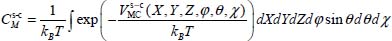
In this expression, kB is the Boltzmann constant,  and
and  (or
(or  for a linear molecule) represent, respectively, the position of the center of mass G and the instantaneous orientation of the trapped molecule (Figure 3.4). Note that, given the asymmetry of clathrate nano-cages, the force field acting on the trapped species cannot be considered spherical; no analytic integration is possible. In addition, the orientational motion of the trapped species cannot be considered as a free rotational motion.
3.4.2. Determination of the Langmuir constants
To determine the Langmuir constant associated with a species trapped in a cage and at a given temperature, it is necessary to numerically construct the potential hypersurface at six degrees of freedom (five for a linear molecule) corresponding to all configurations of the molecule relative to the fixed reference frame linked to this clathrate cage. This also makes it possible to determine the equilibrium configuration, at zero temperature, associated with the minimum  interaction potential energy.
In addition, the formation of clathrates can occur under greatly varying temperatures; we propose to express the Langmuir constant in the simple van’t Hoff form, already used by Bazant and Trout [BAZ 01] and Anderson et al. [AND 05], and in a temperature range between 50 and 300 K:

where  and
and  are adjustment constants of the numerical values obtained from the expression [3.6]. The van’t Hoff expression [3.7] can, for example, be used by the planetology community concerning solar system bodies.
3.4.3. Application to triatomic molecules
Four triatomic species of atmospheric and astrophysical interest are considered in this study: carbon dioxide (CO2), a linear symmetric molecule; hydrogen cyanide (HCN), a linear asymmetric molecule; sulfur dioxide (SO2) and hydrogen sulfide (H2S), both nonlinear symmetric molecules. Table 3.3 presents the geometric characteristics of these molecules and their charge distribution used in our calculations [SPA 86, KET 11, PAR 07].
Table 3.3. Geometric characteristics and electric charge distributions in the molecules studied
3.4.3.1. Conditions and calculation steps
As mentioned above, the clathrate matrices used in our calculations consist of 2,944 water molecules in the case of the sI structure and 3,672 water molecules in the case of the sII structure.
In each “trapped molecule–clathrate matrix”, the first step consists of preliminary calculations of interaction energies in order to define the intervals and not the variation in the different degrees of freedom of the molecule, so that the variation in energy associated with the various configurations is small; this ensures that the value of this energy does not exceed a limit value chosen according to the considered “trapped molecule–clathrate matrix”.
The second step consists of minimizing the interaction energy with respect to the coordinates of the center of mass G of the molecule and its angular coordinates, thus leading to the equilibrium configuration. This also reveals the preferential structure associated with the trapped species.
The equilibrium configuration  and the corresponding minimum energy
  of each of the trapped species are presented in Tables 3.4−3.7.
Table 3.4. Equilibrium configurations and minimum energies of the linear symmetric molecule CO2 trapped in a “s-c” clathrate matrix, s = sI or sII and c = s or l
| CO2-sI-small | CO2-sI-large | CO2-sII-small | CO2-sII-large | |
| Xe (Å) | 0 | 0 | 0.05 | −0.15 |
| Ye (Å) | 0 | −0.35 | −0.10 | −0.90 |
| Ze (Å) | 0 | −0.35 | −0.05 | 0 |
| φe (deg.) | 115 | 110 | 70 | 170 |
| θe (deg.) | 90 | 130 | 70 | 120 |
 |
−275.3 | −371.9 | −214.2 | −302.3 |
Table 3.5. Equilibrium configurations and minimum energies of the linear asymmetric molecule HCN trapped in a “s-c” clathrate matrix, s = sI or sII and c = s or l
| HCN-sI-small | HCN-sI-large | HCN-sII-small | HCN-sII-large | |
| Xe (Å) | 0 | −0.40 | 0 | 0.60 |
| Ye (Å) | −0.30 | 0.40 | −0.30 | −0.80 |
| Ze (Å) | 0 | −0.20 | −0.15 | 0.40 |
| φe (deg.) | 90 | 240 | 70 | 210 |
| θe (deg.) | 150 | 10 | 70 | 120 |
 |
−364.4 | −387.6 | −241.5 | −239.6 |
Table 3.6. Equilibrium configurations and minimum energies of the nonlinear symmetric molecule SO2 trapped in a “s-c” clathrate matrix, s = sI or sII and c = s or l
| SO2-sI-small | SO2-sI-large | SO2-sII-small | SO2-sII-large | |
| Xe (Å) | 0 | −0.15 | 0 | 0 |
| Ye (Å) | 0 | 0 | −0.15 | −0.80 |
| Ze (Å) | −0.40 | 0.45 | 0.30 | −0.20 |
| φe (deg.) | 30 | 0 | 75 | 75 |
| θe (deg.) | 0 | 165 | 165 | 90 |
| χe (deg.) | 90 | 80 | 10 | 60 |
 |
−399.3 | −557.6 | −143.3 | −371.4 |
Comparing the minimum energy  values associated with each “trapped-molecule–cage-structure” considered system clearly shows that the four molecules preferentially trap in small and large cages of the structure type sI. In fact, the values
  in the first two columns of each table are much lower than those in the last two columns. In addition, note that the center of mass of each molecule is not situated in the center of the occupied nano-cage.
Table 3.7. Equilibrium configurations and minimum energies of the nonlinear symmetric molecule H2S trapped in a “s-c” clathrate matrix, s = sI or sII and c = s or l
| H2S-sI-small | H2S-sI-large | H2S-sII-small | H2S-sII-large | |
| Xe (Å) | 0 | −0.20 | 0.15 | 0.6 |
| Ye (Å) | 0 | 0.40 | −0.30 | −0.6 |
| Ze (Å) | −0.40 | −0.80 | −0.30 | 0.6 |
| φe (deg.) | 30 | 30 | 120 | 165 |
| θe (deg.) | 0 | 15 | 45 | 75 |
| χe (deg.) | 90 | 0 | 90 | 75 |
 |
−399.2 | −368.6 | −285.4 | −228.9 |
Finally, the last step is to construct the potential hypersurface in order to determine the Langmuir constant and its temperature dependency which is then adjusted in the form of a van’t Hoff function. Table 3.8 shows the parameters  and
and  (expression [3.7]) associated with each “trapped molecule–cage-structure” system in the temperature range 50–300 K.
Table 3.8. Adjustment parameters for the Langmuir constant according to the temperature for different “trapped molecule–cage-structure” systems
| Cage structure | sI-small cage | sI-large cage | sII-small cage | sII-large cage |
| Trapped molecule |  |
 |
 |
 |
| CO2 | 7.776 × 10⁻¹² 2,976.63 | 520.558 × 10⁻¹² 4,674.69 | 7.997 × 10⁻¹² 2,277.757 | 6,907.001 × 10−12 3,370.363 |
| HCN | 7.665 × 10⁻¹² 4,085.369 | 131.161 × 10⁻¹² 4,328.556 | 13.914 × 10⁻¹² 2,593.031 | 8,224.513 × 10−12 2,640.868 |
| SO2 | 1.231 × 10⁻¹² 4,374.084 | 75.064 × 10⁻¹² 6,272.810 | 6.152 × 10⁻¹² 1,548.504 | 17,926.753 × 10−12 4,139.948 |
| H2S | 234.440 × 10⁻¹² 4,463.910 | 720.800 × 10⁻¹² 4,073.045 | 364.150 × 10⁻¹² 3,073.324 | 75,835.750 × 10−12 2,495.937 |
3.5. Infrared spectrum of a triatomic in clathrate matrix
3.5.1. Infrared absorption coefficient
The infrared absorption coefficient of a number  of optically active molecules trapped, per volume unit, in matrix at temperature T, is defined as the real part (Re) of the spectral density, in other words the Fourier transform of the time-dependent autocorrelation function Φ(t):

In this expression, ρ(0) is the initial canonical density matrix of the overall system,  is the dipole moment operator of the active molecule defined with respect to the fixed reference frame (see equations [2.50] and [2.55] in Chapter 2), ω is the frequency variable (expressed in wavenumber, cm−1) and c is the vacuum light velocity. The Tr (Trace) symbol denotes the average on the initial conditions at t = 0 and on all the possible evolutions of the system between 0 and t.
In the Heisenberg representation, the dipole moment operator  can be written in the form:
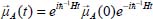
where H is the Hamiltonian of the total system.
3.5.2. Hamiltonian of the system and separation of movements
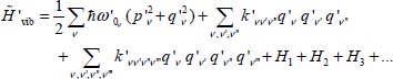
The Hamiltonian of the system consisting of a triatomic molecule in its fundamental electronic state and a clathrate matrix is:

where

is the Hamiltonian associated with the internal vibrational movements, at the harmonic order, of the isolated molecule (gaseous phase), and Tvib is the vibrational kinetic energy operator. The much smaller perturbative Hamiltonians H1, H2, H3 contain the vibrational anharmonicities and the vibrational–rotational interaction of the vibrational potential energy. These terms have been presented in the second section and their terms in Appendix 2.7.2 of Chapter 2.
In equation [3.10], Trot (or Hrot) is the rotational kinetic energy operator (or rotational Hamiltonian) of the isolated rigid molecule (in gaseous phase), introduced in section 4 of Chapter 2. The third term Ttrans of this same expression is the translational kinetic energy operator of the center of mass G of the molecule:

where Pα is the conjugate momentum of translation in the direction α (X,Y,Z) of the fixed reference frame  and M0 is the molecular mass. Finally, HC is the Hamiltonian associated with all degrees of freedom of water molecules in the clathrate matrix, in the absence (i.e. hypothetical as clathrates form in the presence of a gaseous species) of the trapped molecule, taking into account their internal vibrational, orientational and translational motions (vibration of their respective center of mass).
However, since clathrates are structures that are formed under high pressures and at low temperatures, because of the strong hydrogen bonds between the hydrogen atoms and the oxygen atoms of different water molecules, it is reasonable to initially study the spectroscopic phenomena of the molecule trapped in a supposedly rigid crystal. As a result, the Hamiltonian HC can be ignored in the rest of this chapter.
Moreover, when considering the vibrations of the clathrate nano-cage, we must take into account the possible couplings between these vibrations and those of the trapped molecule. These couplings between vibrations are effective only if conditions of symmetry and resonance are verified as already discussed in Chapter 1, in the context of using the contact method to study vibration–rotation spectroscopy of symmetrical C2v or Cs molecules by Flaud and Camy-Peyret [FLA 81, CAM 85, FLA 90, FLA 13]. Indeed, two vibrations of different symmetries do not undergo resonance, and even if a strong coupling is possible, the phase shift between the vibrational modes destroys this resonance. With regard to the Fermi resonance present in the case of CO2, the matrix to be diagonalized includes only the states of the same symmetry. Similarly, the resonance polyads constructed in the context of the application of the contact method only involve states of the same symmetry. The resonance matrices are block-diagonal and the non-diagonal non-zero elements connect states of the same symmetry. Moreover, at low temperatures, the spectroscopic study may be restricted to cold bands (fundamental transitions) and to low frequencies of clathrate cages. To determine the possible couplings, it is necessary to count the vibrations of the same symmetry with similar frequencies.
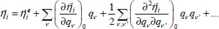
Moreover, the use of the Born–Oppenheimer approximation (adiabatic approximation) makes it possible to separate the high-frequency internal vibrational modes {qv} of the molecule from its low-frequency modes, which are the translational  and orientational
  motions relative to the fixed reference frame
  . The interaction potential energy
  between the molecule and the clathrate matrix can, after a detailed study, be written in the form:

where  is the instantaneous displacement vector of the center of mass of the molecule around its equilibrium position vector
  . In this expression,
  is, as we have seen previously, the value of the energy associated with the equilibrium configuration
  of the rigid molecule in its cage. The second term
  characterizes the orientation and translation movements (movement of the center of mass) of the rigid molecule (low-frequency modes). The third term
  characterizes the internal vibrational motions of the molecule (high-frequency modes) in its equilibrium configuration
  . The experiment shows that this term generally constitutes a small perturbation which causes a displacement and/or a lift degeneracy of the vibrational levels; it can be written in the form of a series development as follows:

where  and
and 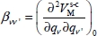 are, respectively, the first and second derivatives of the interaction potential energy
  with respect to the vibrational dimensionless normal coordinates of the trapped molecule.
Finally, the last term 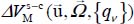 in expression [3.13] characterizes the dynamic coupling between the slow movements (orientation-translation) and the fast movements (vibrations) of the molecule in its cage. This coupling is responsible for possible energy transfers from the vibrational modes to those of translation and orientation (vibrational relaxation phenomenon).
However, an important step in infrared spectrum modeling is the construction of the bar spectrum, that is, determining the integrated intensity and the frequency position of the spectral lines associated with the vibrational–orientational transitions of the optically active molecule. The term  of the expression [3.13] can then be written in the form:

where the first and second terms characterize, respectively, the orientational motion of the trapped molecule in its equilibrium position  and its translational motion (movement of the center of mass) around its equilibrium position, for its equilibrium orientation
  . The last term of expression [3.15] represents the dynamic orientational–translational coupling, responsible for possible energy transfers between the orientational motion and the translational motion (phase relaxation phenomenon), and can therefore induce spectral line broadening.
Finally, this separation of movements or renormalization of the system’s Hamiltonian makes it possible to construct the bar spectrum of the optically active molecule (or optically active vibrational–orientational system) by solving the corresponding Schrödinger equation.
In the Born–Oppenheimer approximation, the Hamiltonian of the optically active system can be written as the sum of a vibrational Hamiltonian and an orientational Hamiltonian:
which can be dealt with separately. The eigenfunctions  of the Hamiltonian
  can be written as the tensorial product
  of eigenfunctions, respectively, of
  and
and  .
.
Note that the rotational constants and the centrifugal distortion constants of the molecule in the gas phase depend on the vibrational state of the molecule. The Schrödinger equation associated with the orientation Hamiltonian  must therefore be solved for each vibrational state involved in a transition.
3.5.3. Vibrational motions
When the molecule is trapped in the clathrate matrix, its nuclei are immersed in a force field, gradient of a perturbed potential function Uvib({qv}):

whose minimum corresponds to a new equilibrium configuration of these nuclei.
Defining this minimum as a new origin of the nuclei motions, we can apply an orthogonal transformation to the vibrational Hamiltonian of the trapped molecule and write:
and by applying the method of contact transformation to the cubic and quartic terms [AMA 57a, AMA 57b], we obtain the energies of the molecule’s vibrational levels perturbed by its environment:

where gv is the degeneracy of the energy level vv, and xvv’ are the anharmonicity constants whose expressions are given in Appendix 2.7.6 of Chapter 2.
Displacements and/or degeneracy lifts of the vibrational levels by the effect of environment can finally be determined.
3.5.4. Orientational motion
In the expression [3.16], the renormalized Hamiltonian  of the orientation motion of the trapped rigid molecule at the equilibrium position of its center of mass is:

Solving of the Schrödinger equation associated with the Hamiltonian,  , making it possible to obtain eigenenergies
  and eigenfunctions
  of orientation, requires a thorough study of the orientational potential energy
  experienced by the molecule trapped in its cage. This model depends on the nature of this orientational motion (free rotation, more or less perturbed rotation, or libration about an equilibrium orientation).
In the case of a linear triatomic molecule, the rotational basis of the isolated molecule and its orientational motion in a nano-cage have been described, respectively, in sections 2.3.2 of Chapter 2 and 4.5.4 of Chapter 4 of Volume 1 [DAH 17], for the study of diatomic molecules.
3.5.5. Translational motion
In a nano-cage, the translation motion of the trapped molecule is no longer free, since it can only perform a translational vibrational motion about its equilibrium position  . In the expression [3.15], the term
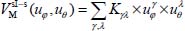
  can be developed as successive power series in terms of uX, uY and uZ in the vicinity of 0. The translational Hamiltonian is therefore written as:
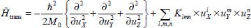
where Klmn are the adjustment coefficients characterizing the forces, the harmonic force constants (quadratic order) and the anharmonic force constants (higher orders) of the translational vibrational motions of the molecule’s center of mass; l, m and n are the natural integers. Note that the coefficient K000 is excluded, since it corresponds to the minimum energy value  .
.
In fact, this series development cannot be done analytically. However, it is possible to numerically build the potential energy surface  that can be adjusted as a polynomial in successive powers of variables uX, uY and uZ and solve the Schrödinger equation associated with the Hamiltonian
  on the basis of an oscillator model.
3.5.6. Bar spectra
The bar spectrum is an important step in the developed model since it gives us information on the quality of the bases associated with the different motions of the “trapped molecule–nano-cage” system and gives an idea of the amplitude of the dynamic coupling between the molecule’s optical vibrational–orientational modes, on the one hand, and the translational vibrational modes of the center of mass of the latter and the motions of water molecules of the clathrate matrix (thermal bath), on the other hand.
The autocorrelation function Φ(t) of expression [3.8] cannot be accurately determined analytically. However, a semi-analytical calculation is possible with certain assumptions and approximations such that:
- – the mean dipole moment induced on the molecule by its inclusion in the nano-cage is negligible;
- – thanks to the renormalization of the system Hamiltonian, the dynamic coupling between the different degrees of freedom, initially small, remains small over time. This justifies the validity of the initial chaos hypothesis (initial decoupling of the optically active system and the thermal bath), making it possible to write the initial canonical density matrix ρ(0) as the product ρopt (0)ρbath(0) of the density matrix associated with the optically active system and that associated with the thermal bath, each being diagonal in its space; and
- – the spectral lines are supposed to be isolated from each other.
Thus, neglecting the dynamic coupling, the integrated absorption coefficient can be written as:
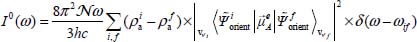
in the case of a pure orientational transition  (far-infrared spectrum), and as:
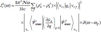
in the case of a vibrational–orientational transition  (near-infrared spectrum).
In the expressions [3.22] and [3.23], 〈...〉 are the transition elements (orientational and vibrational), δ is the Dirac function and ωif is the frequency associated with the transition i → f.  and
and  are, respectively, the optically active populations of the initial and final states involved in the transition. They depend on the energy of the state i (respectively f), the partition function Z, the distribution of optically active molecules over all eigenstates of the Hamiltonian
  and temperature:

where β = 1/kBT, where T is the temperature of the system and kB is the Boltzmann constant.
3.6. Application to the CO2 molecule
In Table 3.4, the equilibrium configuration  and the corresponding minimum energy
  are presented in the case of a CO2 molecule trapped in different nano-cages of clathrate structures sI and sII.
As we can see, the comparison of the minimum energy values  obtained in the different nano-cages clearly indicates that the CO2–sI system with minimum energies calculated at −275 meV and at −372 meV in the small and large cages, respectively, is formed in much more favorable energetic conditions than those of the CO2–sII system with respective energies determined to be −214 meV and −302 meV. These results are consistent with those given by Sloan and Koh [SLO 08].
Thus, in the remainder of this chapter, we will only focus on the spectroscopic study of CO2–sI system. It should be also noted that this molecule is more likely to be trapped in a large cage rather than in a small cage. However, since the clathrates form at a minimum filling rate, we will cover both cases: CO2–sI–small cage and CO2–sI–large cage.
3.6.1. Vibrational motions
As mentioned above, the nuclei of the trapped molecule are immersed in a force field whose minimum corresponds to a new stable equilibrium. The vibrational potential energy function is redefined, by an orthogonal transformation, with respect to this new equilibrium. New constants of harmonic and anharmonic forces must then be determined.
In the case of CO2–sI–small cage, the calculated frequencies of the vibrational modes ν2 and ν3 are shifted towards high frequencies (blue shifted). On the contrary, in the case of CO2–sI–large cage, the values obtained indicate shifts towards the low frequencies (red shifts). However, the spectra observed experimentally indicate low-frequency shifts in both types of nano-cages.
When the trapped molecule is rigid, the effective electrical charges and the Lennard-Jones site-site potential parameters (expressions [3.1] and [3.2]) are accurate enough to allow the calculation of the equilibrium configuration of the molecule and the corresponding minimum energy.
Table 3.9 Frequencies (cm−1) of the normal vibrational modes ν1 ν2 and ν3 of the linear molecule CO2 trapped in the clathrate nano-cages of sI structure
| Vibrational mode | ν1 | ν2 | ν3 | ν3 (13CO2) | |
| ων | Gas | 1,285.4 | 667.4 | 2,349.2 | 2,283.5 |
| ων Calculated | sI–small cage | 1,274.0 | 658.6 659.5 |
2,347.3 | 2,281.6 |
| ων Calculated | sI–large cage | 1,278.0 | 663.3 665.2 |
2,339.7 | 2,274.0 |
| ων Observed | sI–small cage | – | 665 – |
2,347 | 2,280 |
| ων Observed | sI–large cage | – | 659 661 |
2,335 | 2,271 |
On the contrary, when the molecule, taken in its equilibrium configuration, undergoes vibrational motions, the interaction potential energy models applied do not generally lead to values of the vibrational frequency shifts consistent with those observed experimentally. Murchinson et al. [MUR 71a, MUR 71b] and Smith et al. [SMI 72] showed that when a molecule is trapped in a nano-cage, the electron density creating the potential that drives the vibrational motions of the nuclei of this molecule is disturbed in such a way that only the harmonic force constants are significantly modified. A screening effect, through two parameters related to the position of the effective charges in the trapped molecule and its orientation, is then used to adjust the calculated frequency shifts to those observed in the case of the isotope 12CO2–sI–large cage, and thus obtain the modified harmonic force constants which are then used in the case of 12CO2–sI–small cage and for the other isotopes of CO2. Frequency values and the lifting of degeneracy as determined are given in Table 3.9.
3.6.2. Orientational motion
In the case of a linear triatomic molecule, the kinetic energy operator Trot, associated with the rotational motion in the gas phase, involved in the expression [3.20] was presented in the expression [2.82] in Chapter 2 of Volume 1.
Solving the Schrödinger equation associated with the renormalized orientational Hamiltonian  of the rigid CO2 molecule maintained at its equilibrium position in the sI clathrate nano-cages requires a detailed study of the orientational potential energy
  .
.
3.6.2.1. CO2–sI–small cage
In the small cage of the structure sI, the equilibrium configuration of the molecule is obtained when its center of mass is at the center of the cage and its orientation is given by φe = 115° and θ e = 90° (Table 3.4). The corresponding energy is  meV. In Figure 3.5, we present the variation of the orientational potential energy
  in a three-dimensional form (Figure 3.5(a)) and as iso-energy level curves (Figure 3.5(b)). We can see the presence of an orientational symmetry of 180° about φ = 180° and θ = 90°, due to the symmetry of the molecule,
  .
.
The analysis of this potential energy surface shows that the orientation motion has a bi-dimensional (oscillatory) librational character of small amplitudes around the equilibrium orientation of the molecule. The angular coordinates (φ, θ) are no longer suitable for describing this librational motion.
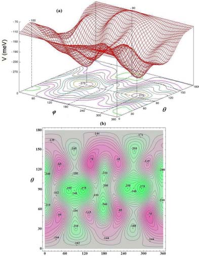
Figure 3.5. Orientational potential energy  (meV) of the molecule CO2 trapped in a small cage of the sI clathrate structure: (a) three-dimensional form and (b) iso-energy level curves. For a color version of this figure, see www.iste.co.uk/dahoo/infrared2.zip
We introduce two new coordinates uθ = cosθ and uφ = φ – φe (uφ expressed in radians) varying about 0. The potential energy  can be adjusted as a series of successive powers of uφ and uθ in the form:
where Kγλ are the adjustment coefficients characterizing the forces, the harmonic force constants (quadratic order) and the anharmonic force constants (higher orders) of the libration motion of the molecule, γ and λ are the natural integers. Note that the term K00 is excluded from this adjustment since it corresponds to the minimum energy value  .
.
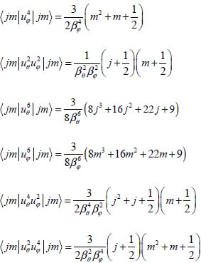
The method to solve the Schrödinger equation  associated with this orientational motion was presented in section 4.5.4.1.3 in Chapter 4 of Volume 1 [DAH 17]. The quantum numbers j and m are associated, respectively, with the librators in θ and φ. In Table 3.10, we limit the given calculated values to the adjustment coefficients obtained up to the order γ + λ = 6.
The values of the pairs (frequency ω coefficient β), calculated at the harmonic order, are (ωφ = 56.9 cm-1, βφ = 8.541) and (ωθ = 101.7 cm-1, βθ = 11.419).
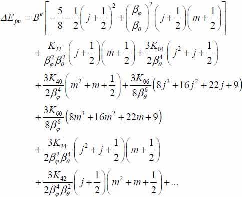
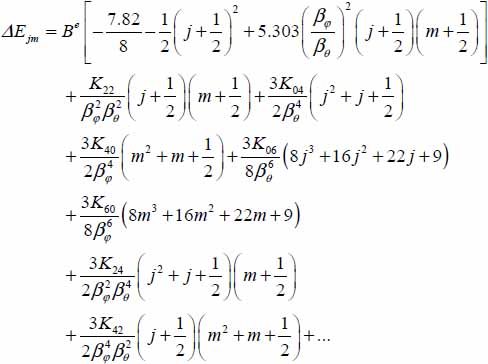
The corrective values of the eigenenergies, obtained using the first-order perturbation method, are included in Figure 3.7(a). The analytical expression of ΔEjm is given in Appendix 3.7.2. Note that at the first-order perturbation, the corrections due to the odd power terms in uθ and uφ are zero. Thus, they were not listed in Table 3.10.
Table 3.10. Adjustment coefficients Kγλ (meV) of potential energy surface in terms of the successive powers of uφ and uθ of the linear molecule CO2 trapped in a small cage of the structure sI. The rotational constant of the molecule is Be = 0.390 cm−1. The energy conversion factor is: 1 meV = 8.06554 cm−1
| K20 | K02 | K40 | K22 | K04 | K60 | K42 | K24 | K06 |
| 257.9 | 822.4 | −293.7 | −1,313.9 | −2,192.6 | −167.2 | 977.0 | 4,480.8 | 3,518.5 |
3.6.2.2. CO2–sI–large cage
When the molecule is trapped in the large cage, it takes an equilibrium position given by Xe = 0, Ye = −0.35 Å and Ze = −0.35 Å which corresponds to an eccentricity  in the OYZ plane parallel to the hexagons of the cage, and an orientation φe = 110° and θe = 130° (Table 3.4). The corresponding energy is
  . In Figure 3.6, we present the variation of the orientational potential energy
  in three-dimensional form (Figure 3.6(a)) and in iso-energy level curves (Figure 3.6(b)). As in the small cage, there is an orientational symmetry of 180° about φ = 180° and θ = 90°, due to the symmetry of the molecule,
  .
.
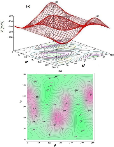
Figure 3.6. Orientational potential energy surface  (meV) of the molecule CO2 trapped in a large cage of the sI Clathrate structure: (a) three-dimensional form and (b) iso-energy level curves. For a color version of this figure, see www.iste.co.uk/dahoo/infrared2.zip
As with the previous case, the analysis of this potential energy shows a librational motion of small amplitudes about the equilibrium orientation of the molecule. We introduce two new coordinates uθ = sin(θ−θe) and uφ = φ − φe (uφ expressed in radians) varying about 0. This is a case that can be found in section 4.5.4.1.4 in Chapter 4 of Volume 1 [DAH 17]. The potential energy  can be adjusted in a successive power series of uφ, and uθ in the form of expression [3.25] where the coefficients of the harmonic terms K20 and K02 are large compared to those of other terms, the eigenvectors |jm〉 of the two-dimensional liberator (oscillator) can be written as the tensorial product of the eigenvectors |j〉 associated with the librator in θ and |m〉 associated with that in φ : |jm〉 = |j〉 ⊗ |m〉.
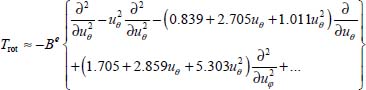
By introducing the new coordinates in the expression of the rotational kinetic energy operator Trot (equation [2.82] in Chapter 2 of Volume 1 [DAH 17]), and after some manipulations and developments as the second-order Taylor series, we obtain the expression:
By putting the equations [3.25] and [3.26] in [3.20], the Hamiltonian  can be written as:
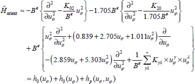
In this expression, the first two terms are the harmonic Hamiltonians associated with the two librators and the third term hp(uθ, uφ) represents the perturbative Hamiltonian analyzed using the stationary perturbation theory. In this last term, the symbol * indicates that K20 and K02 are excluded.
The energy of an eigenstate can be written as:

The eigenenergies  and
and  and the corresponding eigenvectors are:
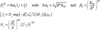
and

where N are the normalization factors and H are the Hermite polynomials. The quantum numbers j and m are the natural integers, independent of each other and are associated, respectively, with the librators uθ and uφ.
Table 3.11 shows the adjustment coefficients obtained up to order γ + λ = 6.
The values of couples (frequency ω, coefficient β), calculated in the harmonic order, are (ωφ = 46.4 cm-1, βφ = 5.907) and (ωθ = 27.9 cm-1, βθ = 5.981).
The corrective values ΔEjm are obtained by applying the first-order perturbation method to the perturbative Hamiltonian hp (uθ, uφ : ΔEjm = 〈jm|hp (uθ, uφ)|jm〉. The matrix elements for determining the analytical expression of ΔEjm are given in Appendix 3.7.2. Note that at the first-order perturbation, the corrections due to the terms of odd powers are zero. The corresponding coefficients are not shown in Table 3.11.
Table 3.11. Adjustment coefficients Kγλ (meV) of the area of potential energy in terms of the successive powers uφ and uθ of the linear molecule CO2 trapped in a large cage of sI structure
| K20 | K02 | K40 | K22 | K04 | K60 | K42 | K24 | K06 |
| 100.6 | 61.9 | −23.4 | −209.6 | 71.5 | 1.8 | 38.8 | 66.0 | −39.3 |
Finally, the calculated values of ΔEjm are included in the level schemes in Figure 3.7(b).

Figure 3.7. Orientational levels of the CO2 molecule trapped in the sI clathrate structure: (a) small cage and (b) large cage
3.6.3. Translational motion
In the small cage, when the molecule is maintained in its equilibrium orientation, its translational potential energy  is almost that of a tri-dimensional harmonic oscillator characterized by small amplitude displacements about the center of the cage.
In the harmonic approximation, solving the Schrödinger equation associated with the Hamiltonian  (equation [3.21]) gives the frequencies ωX = 95 cm-1, ωY = 125 cm-1 and ωZ = 115 cm-1.
In the large cage, when the molecule is maintained in its equilibrium orientation, its translational potential energy  characterizes two oscillators around the equilibrium position Xe = 0, Ye = −0.35 Å and Ze = −0.35 Å: i) the first along the X-axis perpendicular to the two hexagons of the cage, with small-amplitude harmonic oscillations; and ii) the second in the XY plane (neither along axis Y nor axis Z) with large-amplitude anharmonic oscillations.
In the harmonic approximation, the frequencies obtained are ωX = 55 cm-1 and ωYZ = 29 cm-1.
3.6.4. Bar spectra
We have seen that CO2 molecules can stabilize the sI clathrate structure in small or large cages. The number  of optically active molecules per volume unit (equation [3.8]) can be written as the sum
  of the number of optically active molecules trapped, per volume unit, in small or large cage, respectively.
Since CO2 is a linear symmetric molecule, it does not have a permanent dipole moment μe = 0. Therefore, no pure orientational transition can take place, so there is no far-infrared spectrum. In addition, its symmetric vibrational mode ν1 (symmetric stretch) is inactive in the near-infrared range.
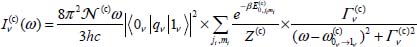
Thus, the integrated near-infrared absorption coefficient of the  trapped active molecules, per volume unit and at temperature T, in cages c (c = s or 1) and associated with the transition |0ν〉(c) → |1ν〉(c) of mode ν (the other modes being in their fundamental state), is written as:
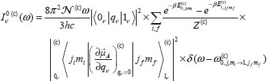
 is the frequency associated with the transition |0ν, jimi〉(c) → |1ν, jfmf〉(c). Given the large eigenenergies of the excited vibrational states and the low temperatures considered in this study, populations of active molecules
  (see equation [3.24]) in these states are negligible.
Moreover, in the harmonic approximation of the normal vibrational modes of the trapped molecule, the vibrational transition elements are given by  .
.
In the orientational transition elements of equation [3.31], the expression of the vector  with respect to the reference frame
  linked to the molecule was given in equation [2.55] in Chapter 2. In the case of the CO2 molecule, Table 3.12 presents the values of the first derivatives of the components of the dipole moment, with respect to the equilibrium configuration reference frame
  of the molecule, associated with its vibrational modes.
Table 3.12. First derivative values of components of the dipole moment, with respect to the equilibrium configuration reference frame  of 12CO2, associated with its vibrational modes: ν1 symmetric stretching, ν21 and v22 bending (angular deformation) and ν3 asymmetric stretching. The values in parentheses are for the isotope 13CO2
| Modes | ν1 | ν21 | ν22 | ν3 |
 |
0 (0) | −0.184 (−0.178) | 0 (0) | 0 (0) |
 |
0 (0) | 0 (0) | −0.184 (−0.178) | 0 (0) |
 |
0 (0) | 0 (0) | 0 (0) | 0.461 (0.448) |
The expressions of the vector components  associated with the different vibrational modes of the molecule are given in Appendix 3.7.3, and those of the orientational transition elements of the molecule trapped in small or large clathrate cages are given in Appendix 3.7.4.
The calculation of these transition elements shows that ~ 98% of the transitions are pure vibrational transitions |0ν, jm〉(c) → |1ν, jm〉(c) and the remaining ~ 2% are librational–vibrational transitions |0ν, jimi〉(c) → |1ν, jfmf〉(c) which, therefore, will be ignored. The near-infrared spectra associated with the vibrational modes ν2 and ν3 are composed of pure vibrational spectral lines.
For the isotope 12CO2, in the frequency region of mode ν3, we obtain two spectral lines of integrated intensities  and
and  (in arbitrary unit) at 2,347.3 and 2,339.7 cm−1 associated, respectively, with the molecules trapped in small and large cages. Whereas for the isotope 13CO2, we obtain two spectral lines of integrated intensities
  and
and  (in arbitrary unit) at 2,281.6 and 2,274.0 cm−1 associated, respectively, with the molecules trapped in small and large cages.
Comparing these calculated intensities with existing experimental spectra of Fleyfel and Devlin [FLE 91] and Dartois and Schmitt [DAR 09] requires the knowledge of the  and
and  distribution of active molecules in small and large cages of the sI clathrate structure.
However, using the Lorentzian model of spectral lines (equation [4.109] in Chapter 4 of Volume 1 [DAH 17]), the integrated intensity can be written as:
where  is the linewidth at half height. It is then possible to determine the distribution
  and
and  by calculating the ratios
  of the integrated intensities associated with the ν3 mode, respectively, in large and small cages, with
  and
and  where
where  are deduced from experimental spectra. The ratios
  are then calculated and adjusted to the corresponding experimental data.
In the case of isotope 12CO2, the distribution obtained is  and
and  using the spectrum of Fleyfel and Devlin [FLE 91] at temperature T = 13 K.
In the case of isotope 13CO2, the calculated distributions are  and
and  using the spectrum of Fleyfel and Devlin [FLE 91] at T = 13 K, on the one hand, and
  and
and  using the spectrum of Dartois and Schmitt [DAR 09] at T = 5.6 K, on the other hand.
As we can see, in spite of the approximate nature of the Lorentzian model, the distributions obtained are fairly similar and consistent with the distribution of small and large cages of the sI clathrate structure, that is, two small and six large cages per unit cell.
Thus, with this distribution, it is possible to predict the line intensities in the frequency region of the vibrational mode ν2 (doubly degenerate bending mode) of 12CO2.
The spectrum obtained consists of two lines with an intensity of 2.8 (in arbitrary unit) at frequencies 658.6 cm−1 and 659.5 cm−1 for the molecules trapped in small cages and two lines of intensity 8.4 (in arbitrary unit) at frequencies 663.3 cm−1 and 665.2 cm−1 for the molecules trapped in large cages, which is due to the degeneracy lifting of this mode in anisotropic nano-cages.
3.7. Appendices
3.7.1. Non-zero orientation matrix elements used to calculate the corrections to first-order perturbation energies

3.7.2. Correction to eigenenergies of the orientation Hamiltonian
3.7.2.1. CO2–small cage
FORTRAN Program
C********************************************************************
C*Program co2nivlib.f <=====>
C*CALCULATION OF ORIENTATIONAL ENERGY LEVELS IN THE CASE OF A
C* LINEAR MOLECULE
C*THETA LIBRATION MOTION ABOUT Pi/2
C* PHI LIBRATION MOTION ABOUT AN EQUILIBRIUM VALUE
C*==> BASE PROCESSING OF HARMONIC LIBRATOR
C* PERTURBATION ORDER 1
C********************************************************************
C The perturbation is considered up to order 6
   B= 0.39        ! Cste rotational in cm-1
   DK20= 2079.8       ! in cm-1.rad-2
   DK02= 6633.0       ! in cm-1
   DK40= - 2368.8     !……
   DK04= -17684.9
   DK22= -10597.8
   DK60= - 1348.3
   DK06= 28378.4
   DK42= 7880.3
   DK24= 36140.5
   hnuthe= 2.*SQRT(B*DK02)   ! hnu = hbaromega
   hnuphi= 2.*SQRT(B*DK20)
   betthe= SQRT(SQRT(DK02/B))
   betphi= SQRT(SQRT(DK20/B))
   WRITE(*,1958)hnuthe,hnuphi,betthe,betphi
1958 FORMAT(/10X,'hnuthe =',F10.3,15X,'hnuphi =',F10.3//9X,'betathe ='
   &,F10.5,14X,'betaphi =',F10.5///)
   WRITE(*,1996)
1996 FORMAT(6X,'j',6X,'m',8X,'E0j',10X,'E0m',11X,'EPjm', &7X,E0Pjm (cm-1)'//)
   DO j=0,4
   DO m=0,4
C**********************************************************
   E0j= hnuthe*(j+1./2.)
   E0m= hnuphi*(m+1./2.)
   EPjm= B*(-0.5*j*j-0.5*j-0.75+0.25*(2.*j+1.)*(2.*m+1.)
   & *betphi*betphi/betthe/betthe)
   & +0.25*(2.*j+1.)*(2.*m+1.)*DK22/
   & betphi/betphi/betthe/betthe
   & +0.75*(2.*j*j+2.*j+1.)*DK04/(betthe**4)
   & +0.75*(2.*m*m+2.*m+1.)*DK40/(betphi**4)
   & +0.375*(8.*j*j*j+16.*j*j+22.*j+1.)*DK60/(betthe**6)
   & +0.375*(8.*m*m*m+16.*m*m+22.*m+1.)*DK06/(betphi**6)
   & +0.375*(2.*j*j+2.*j+1.)*(2.*m+1.)*DK42/(betthe**4)/
   &              (betphi**2)
   & +0.375*(2.*j+1.)*(2.*m*m+2.*m+1.)*DK24/(betthe**2)/
   &              (betphi**4)
   E0Pjm= E0j+E0m+EPjm
C**********************************************************
   WRITE(*,1961)j,m,E0j,E0m,EPjm,E0Pjm
1961 FORMAT(2(5X,I2),4(5X,F8.2))
   ENDDO
   ENDDO
   STOP
   END
C********************************************************************
3.7.2.2 CO2–large cage
FORTRAN Program
C**********************************************************
C*Programme co2nivlib.f <=====>
C* CALCULATION OF ORIENTATIONAL ENERGY LEVELS IN THE CASE OF A
C*       LINEAR MOLECULE
C*THETA LIBRATION MOTION ABOUT Pi/2
C*PHI LIBRATION MOTION ABOUT AN EQUILIBRIUM VALUE
C*==> BASE PROCESSING OF TWO HARMONIC LIBRATORS
C* PERTURBATION ORDER 1
C**********************************************************
C The perturbation is considered up to 6
   B= 0.39   ! Cste rotational in cm-1 ---> Mvt in theta
   Bphi= 1.704*B ! Attention Bphi   ---> Mvt in phi
   DK20= 811.0       ! in cm-1.rad-2
   DK02= 498.9       ! in cm-1
   DK40= - 188.7     !……
   DK04= 576.5
   DK22= - 1690.1
   DK60= 0.0
   DK06= - 317.2
   DK42= 312.9
   DK24= 532.2
   hnuthe= 2. *SQRT(B*DK02)    ! hnu = hbaromega
   hnuphi= 2.*SQRT(Bphi*DK20)
   betthe= SQRT(SQRT(DK02/B))
   betphi= SQRT(SQRT(DK20/Bphi))
   WRITE(*,1958)hnuthe,hnuphi,betthe,betphi
1958 FORMAT(/10X,’hnuthe = ‘,F10.3,15X,’hnuphi = ‘,F10.3//9X,’betathe =‘
   &,F10.5,14X,’betaphi =‘,F10.5///)
   WRITE(*, 1996)
1996 FORMAT(6X,’j’,6X,’m’,8X,’E0j’,10X,’E0m’,11X,’EPjm’,
   &7X,’E0Pjm (cm-1)’//)
   DO j=0,6
   DO m=0,6
C**********************************************************
   E0j= hnuthe*(j+1./2.)
E0m= hnuphi*(m+1./2.)
EPjm= B*(-0.5*j*j-0.5*j-1.102+1.326*(2.*j+1.)*(2.*m+1.)
   & *betphi*betphi/betthe/betthe)
   & +0.25*(2.*j+1.)*(2.*m+1.)*DK22/
   & betphi/betphi/betthe/betthe
   & +0.75*(2.*j*j+2.*j+1.)*DK04/(betthe**4)
   & +0.75*(2.*m*m+2.*m+1.)*DK40/(betphi**4)
   & +0.375*(8.*j*j*j+16.*j*j+22.*j+1.)*DK60/(betthe**6)
   & +0.375*(8.*m*m*m+16.*m*m+22.*m+1.)*DK06/(betphi**6)
   & +0.375*(2.*j*j+2.*j+1.)*(2.*m+1.)*DK42/(betthe**4)/
   & (betphi**2)
   & +0.375*(2.*j+1.)*(2.*m*m+2.*m+1.)*DK24/(betthe**2)/
   & (betphi**4)
   E0Pjm= E0j+E0m+EPjm
C**********************************************************
   WRITE(*,1961)j,m,E0j,E0m,EPjm,E0Pjm
1961 FORMAT(2(5X,I2),4(5X,F8.2))
   ENDDO
   ENDDO
   STOP
   END
C*************************************************************
3.7.3. Expressions of the vector components derivatives of the dipole moment with respect to the normal vibrational coordinates
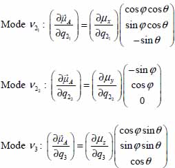
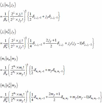
3.7.4. Expressions of the orientational transition elements in the approximation of harmonic librators
The second-order series development of trigonometric functions cos φ, sin φ, cos θ and sin θ in terms of the variables uφ and uθ introduced in the study of orientational motions of the molecule trapped in small and large cages (section 3.6.2) allows us to obtain the expressions of dipolar transition elements. The selection rules associated with these variables are also presented below.
3.7.4.1 CO2–small cage
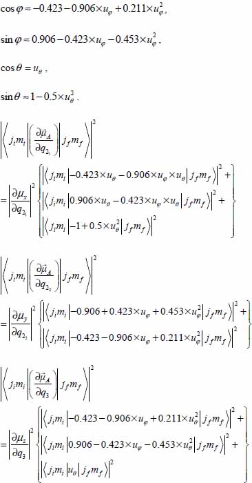
The selection rules associated with the variables u are:
with βφ = 8.541 and βθ = 11.419.
3.7.4.2. CO2– large cage
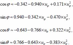

The selection rules associated with the variables u are identical to the previous ones, with βφ = 5907 and βθ = 5.981.