16 Failure
In parts I and II, we considered computations running on perfect step-taking machinery. That doesn’t mean we’ve considered only perfect computations: we’ve been concerned with flaws, especially wrong specifications or wrong implementations, and we’ve also been concerned with not having enough resources for a computation. But so far we haven’t been concerned with what to do when the machinery breaks, or just doesn’t work correctly any more.
By thinking about how systems fail, we can build systems that tolerate or overcome failures. We need to understand something about the likelihood of failures, and the shape or form of the failures, so as to be able to build systems that can keep working in spite of those failures. We can move our systems toward being unstoppable.
Reliability vs. Availability
Assume that we have some valuable service like the Google search service, and we’d like for it to have this unstoppable quality. There are two often confused issues involved, which computer scientists call reliability and availability.
Reliability refers to the integrity of the service—correctness of the answers we get, durability of any state that’s maintained—but doesn’t say anything about whether the system actually provides the service. Having a service that is only reliable is like having a very trustworthy friend with an unpredictable schedule—you’re not quite sure whether you’ll be able to get hold of them, but you know that they will absolutely be able to give you the right answer if you can find them. In figure 16.1 we show the trustworthy friend present in some boxes and absent in others.
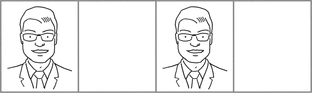
High reliability, low availability.
In the context of the Google search service, reliability means that the search results are high quality and not subject to losses or strange variations every time some component has failed. However, the service might be completely unable to give an answer, in which case its theoretical reliability is not very relevant.
In contrast, availability refers to the likelihood of getting service, while saying nothing about the quality of the service—like whether the answer received is correct. Having a service that is only available is like having a friend with poor judgment who nevertheless keeps a very predictable schedule; you always know exactly when and where to find them, but whether they can help you with your problem is hit-or-miss. In figure 16.2 we show someone present in every box, but most of the time he’s kind of goofy and not very helpful.

High availability, low reliability.
In the context of the Google search service, availability means that the service is always willing to answer search requests. However, those answers might be dubious or just plain wrong, in which case the service’s conspicuous availability is not very relevant.
Table 16.1 is another way of summarizing the difference between reliability and availability.
Reliability vs. Availability
Likelihood of getting some answer |
Likelihood of getting a good answer |
|||
Reliable |
? |
High |
||
Available |
High |
? |
Ideally we would design systems to be both reliable and available in all cases—like a trustworthy friend with consistent habits. That’s what we show in figure 16.3 with the “good” version in every box.
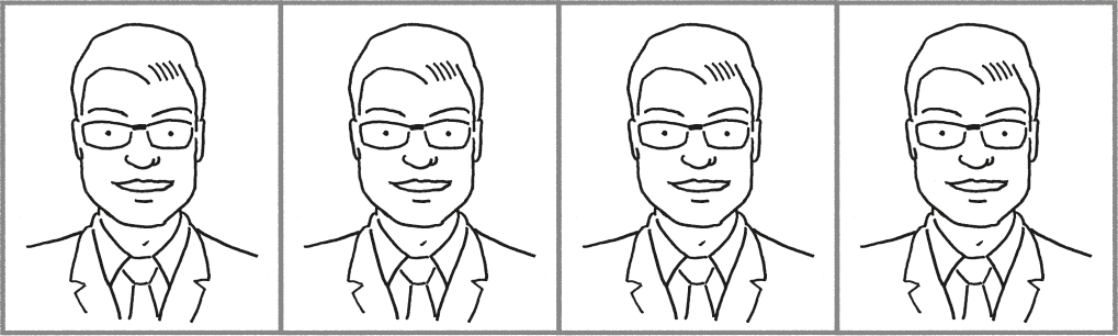
The ideal: high reliability and high availability.
Unfortunately, in the presence of failures we often have to trade off one characteristic against the other.
Fail-Stop
In the most common approach to handling failure, we assume that each component either works correctly or fails completely (falls silent, dies) – nothing in between. A computer scientist would call this approach a fail-stop model.
In this model, it doesn’t matter how simple or complex the machine is; it’s either working or broken. The fail-stop model is essentially a variant of the digital model that we saw in chapter 2. The digital model separates all real-world variability and fuzziness into just the two values “0” and “1.” Correspondingly, the fail-stop model separates all of the messiness of possible operating conditions into just two distinct states, which are usually called “up” and “down.” “The system is up” means that it’s working, while “the system is down” means that it’s failed. In much the same way that a digital model doesn’t recognize the validity of a halfway extended state for a counting finger, the fail-stop model doesn’t recognize any sort of “mostly working” or “limping along” situation for step-taking machinery. Sometimes people talk about a computer, program, or disk crashing. For example, “my laptop crashed,” or “the mail server crashed.” That terminology is usually an indication that they are referring to a system built around a fail-stop model.
A fail-stop model acknowledges that the universe is imperfect—things do fail unpredictably. However, a fail-stop model implies that apart from those unpredictable failures, the universe is pretty well behaved. There are other failure models that allow for a more pessimistic view—seeing the universe as more hostile. We’ll mention one of these other models in chapter 17.
Spares
In a fail-stop world, we need to have multiple copies of computers and storage if we want to have an unstoppable system, because any single copy can fail; and the failure might be permanent. For example, a computer can simply stop working—either because it has no power, or because something else has gone wrong that effectively looks like losing power. Similarly, a storage device can simply stop working, which means that we’ve lost whatever was stored there … unless we kept another copy of that data somewhere else. So in a fail-stop world, we need to assemble multiple computers and/or multiple storage devices in ways that allow the system to tolerate failures.
Computer systems aren’t the only place where we might encounter multiple redundant copies. The most familiar version of this same principle in everyday life is to simply have a spare. For example, most cars carry a spare tire mounted on a spare wheel. If one of the car’s tires is damaged so that it can’t work anymore (for example, it’s been punctured so that it can’t hold air), then the bad wheel is removed and the spare wheel replaces it. Similarly, a car rental location typically has more cars available than are actually committed to renters at any given time. If you’re picking up a rental car and the first car assigned is unsatisfactory for some reason, it’s usually not too hard to swap in another car as a replacement.
The idea of spares and recovery can also be applied at much finer granularity, and in particular we can have “spare bits” to help recover from “failed bits.” Just as words can get garbled or lost by noise in ordinary conversation, and papers can get lost or decay in storage, we can be in a situation where some particular bit is unclear, and we can no longer tell whether the value of that bit should be 0 or 1.
Using spares to solve this problem may seem a little weird—we can’t just literally supply a single “spare bit” like a spare tire, of course. We don’t know in advance what the bit value is that we’ll have to replace. And keeping two spare bits so we have both values available isn’t an improvement! If we have two spare bits, one 0 and one 1, we know in an annoying-mathematician way that we definitely have the right replacement value available. We just don’t know which one it is, which is sort of useless. So using spare bits is not quite like the spare tire approach.
Error Correction
Instead, we can think of supplying enough additional information so that we can reconstruct the lost bit. The situation is like a tiny detective story in which we figure out the original value by examining the clues left in the aftermath of the failure. In contrast to a typical detective story, we’re not trying to figure out the identity of the perpetrator; instead, we’re trying to figure out the identity of the victim, the missing bit.
Here’s a really simple and inefficient version: if we knew in advance that we would only ever lose one bit at a time, and we weren’t very worried about costs, we could simply use two bits for every original bit. That is, instead of transmitting/storing “1” we would transmit/store “11.” Likewise, instead of “0” we would use “00.” Table 16.2 summarizes that information.
If we’re using this scheme, then when some bit was garbled or noisy so we couldn’t understand it (which we’ll write as “?”) we would wind up with a 2-bit sequence like “1?” (1 followed by not-sure) or “?0” (not-sure followed by 0). In either of those cases, we would be able to rebuild the right value by using the bit that didn’t get garbled. Table 16.3 summarizes the value reconstruction by the receiver.
Simple bit-doubling code: receiver’s actions
When we receive… |
It really means… |
||
00 |
0 |
||
0? |
0 |
||
?0 |
0 |
||
11 |
1 |
||
1? |
1 |
||
?1 |
1 |
This bit-doubling is a very crude example of an error-correcting code. In practice, this particular code has two problems: first, it takes up twice as many bits as the information that we are actually transmitting, so all of our storage and transmission costs double. Second, even after taking up twice as many bits, the code will only work correctly if a single bit at a time changes, and only to a “not-sure” state. If there is ever any scenario in which more than one bit can change at once, or a bit could change to its opposite value, this simple code doesn’t help. It could either leave us unsure about the value (a pair like “??” could represent either 0 or 1), or worse it could flip a bit undetectably (producing a pair like “11” when the original value was “00,” for example).
Fortunately, there are more sophisticated codes that perform much better, requiring only a small “tax” of extra bits to handle larger and more complex failure cases.
Error Detection
We’ve just looked at a simple example of an error-correcting code. It’s also possible to have a weaker kind of “spare bit” scheme called an error-detecting code. An error-detecting code only lets us know that something has gone wrong, but doesn’t supply the right answer.
For example, our simple bit-doubling code works as an error-correcting code if we know that only one bit can be wrong. However, if we use that exact same code in an environment where there could be two errors in a row, the code is no longer able to correct all errors that occur. In particular, when two errors produce the code “??” we can tell that’s not a good answer—but we can’t tell what it should have been.
In general, we would prefer to get the right answer rather than just knowing there’s been a mistake. So why is an error-detecting code ever interesting? There are two basic reasons. One possibility is that a correction isn’t useful; the other possibility is that a correction isn’t possible. We’ll explain both these cases a little further.
We might think that a correction is always useful, but sometimes a low-level failure requires a high-level reset or restart. It’s not always useful to fix the immediate problem. For a real-life analogy, consider booking travel. If your desired flight is sold out, it may or may not make sense for you to be booked onto an alternative. Under some circumstances, another flight may be a fine substitute; in other cases, the inability to get a particular flight may mean the whole itinerary needs to be reworked, or the whole trip needs to be scrapped. An “error-correcting” travel agent who always gets us from point A to point B regardless of the date, time, or airline may be unhelpful or even aggravating.
Likewise in a computation: if some or all of the preceding steps need to be redone, there may well be completely different data being handled, and the recovery of the garbled data is pointless. Under these circumstances, it may be useful to perform error detection just to be aware that the data is not correct. However, it would be unwise to incur any additional cost to achieve local error correction. We will encounter a more-general version of this line of thought in chapter 18, where it is an important design principle for reliable communication.
The other reason for wanting error detection is that it’s an improvement over having nothing, in cases where error correction is not possible. Any error-correcting code has some limit on the number of errors that it can correct. Any error-detecting code likewise has some limit on the number of errors that it can detect. However, in general it is easier to detect errors than to correct them, as we have already seen with our simple bit-doubling code: it can still detect a kind of error that it can’t correct.
To understand these levels of difficulty, let’s look again at a concrete example. Assume that errors never flip 0 directly into 1 or vice-versa, but always go through “?” first. How does our bit-doubling approach perform for error correction and detection in that environment? It’s a code that can correct one bad bit, can detect two bad bits, but can’t detect three or more bad bits. Any single error can be one of the following four changes, where we use a right arrow → to mean “becomes”:
0 → ?
? → 0
1 → ?
? →1
but a single error cannot be one of the following two changes:
0 → 1
1 → 0
Under these assumptions, our simple bit-doubling code offers different “levels” of capability, depending on how many errors have occurred. We can distinguish the following four levels in terms of a sequence of flips applied as we try to transmit the single bit value “1”:
• 0 errors: Normal operation, correct result decoded
Example: We send “11” which is received as “11” and correctly decoded as “1”
• 1 error: Error-correcting operation, correct result decoded
Example: We send “11” which is corrupted to “1?” but still correctly decoded as “1”
• 2 errors: Error-detecting operation, result may be incorrect but is known to be flawed
Example: We send “11” which is corrupted to “1?” and then further corrupted to “??” which can’t be reliably decoded. But the receiver knows that an error has occurred.
• 3 or more errors: Erroneous operation, result may be incorrect and may not be known to be flawed
Example: We send “11” which is corrupted to “1?” and then further corrupted to “??” and yet further corrupted to “?0” which is incorrectly decoded as “0”
Keep in mind that this simple bit-doubling code is intended to be easy to understand, not to work efficiently. More realistic codes work differently. However, this overall pattern is typical: increasing the number of errors shifts the system successively from normal operation to error-correcting operation (if possible), then to error-detecting operation (if possible), and finally to erroneous operation.
Storage and Failure
Ideas about error correction and error detection are not only useful for the transmission of data; they are also applicable to the storage of data. This similarity is not surprising if we engage in some big-picture thinking: after all, storage is effectively just a transmission to some future recipient (possibly our future self), while retrieval of stored information is just receipt of a transmission from a past sender (possibly our past self).
In addition to error-detecting and error-correcting codes, there are other kinds of spares or redundancy that we can use to build reliable storage systems. Before we look at those approaches, it’s worth understanding a little about what’s happening in storage and what’s failing.
At this writing, large-scale, long-term storage is typically on magnetic disks. They have a thin layer of material that can be selectively magnetized so as to encode information in the patterns of magnetization, and the pattern of magnetization can then be sensed to read back the information that was encoded there. The underlying magnetic technology is similar to what was used to record music on audio cassettes and 8-track tapes—formats that were once popular but are now obsolete. However, the similarity is only in the use of magnetic techniques. Those old music formats used magnetic storage to record music in analog form. In contrast, we want to record digital data (recall that we looked at analog vs. digital models in chapter 2).
In principle, magnetic storage is not very different from what you can do with paper, pencil, and eraser: making marks and reading them later. That said, there are some useful differences. It’s handy that the magnetic “marks” being made are tiny, which means that a small device can store a very large number of them. It’s also handy that the “pencil” and the “eraser” are combined. The effect is a little like having one of those pens that lets you click among different points with different ink colors—except that instead of having one blue point and one red point, here one point marks and one point erases. Finally, magnetic writing and erasing causes far less wear than the corresponding operations with pencil and eraser, so a magnetic storage device can still be working fine long after a cycle of repeated writing and erasing that would wear out even the best paper.
Although they’re superior to writing and erasing paper, magnetic disks are usually the least reliable elements of computer systems. This is not because the manufacturers are incompetent, but because magnetic disks involve a kind of mechanical brinksmanship. People want magnetic disks to have both fast operations and high density (many bits of storage per device). It’s expensive to build the mechanism that reads and writes bits magnetically, so that element is just a small read/write head that operates on only a tiny fraction of the total storage at any one time. To read or write something on a part of the disk far away from the current position of the read/write head, the head and/or the disk has to move so that the head is directly over the area of interest.
Although we’re currently focused on magnetic disks, we can note in passing that there’s a similar structure to both vinyl phonograph records and optical CDs or DVDs. In all of these systems, there’s a relatively large rotating disk containing information of interest, but only a relatively small area where the “action” happens.
In fact, it’s useful to pursue this comparison a little further and consider what’s happening “up close” with a record, a CD/DVD, and a magnetic disk.
In figure 16.4, we see a section through the playback mechanism using vinyl records. The stylus actually rests on the record. Although this wears out the vinyl, the stylus is very light and the record doesn’t move very fast.

Cross section of vinyl record in use.
In figure 16.5, we see a similar view but now of a CD or DVD. The read/write mechanism is optical, based on lasers. There is no longer any need for physical contact, and instead there’s an emphasis on moving the disk quickly. To achieve fast operations, there needs to be only a short time between when a request is made and when the read/write head is in the right part of the disk. To minimize that delay time, the disk needs to spin rapidly. A rapidly spinning disk moves the relevant areas quickly under the read/write head where the “action” occurs.

Cross section of optical disk (CD/DVD) in use.
Similar reasoning applies to a magnetic disk, but there is an additional constraint. To achieve high storage density, the units of magnetization that represent bits must be very small. Using small units means that the magnetic force to be sensed is small, which in turn means that the read/write head must be positioned very close to the magnetic material, as shown in figure 16.6.

Cross section of magnetic disk in use.
Fast operations and high density mean that we have to have the disk spinning as fast as possible, with the head as close to the disk as possible. The combination of a fast-moving disk and a very close head means that there is no room for mechanical error or wear.
Flash
Magnetic storage is not the only way to store a large number of bits so that they can still be read days, weeks, or years later. Especially in phones and other mobile devices, it is more common to use flash or solid state drives that have no mechanical moving parts, just as the other elements of most computer systems have no mechanical moving parts. Instead of “marking” tiny magnetic areas, these technologies “mark” an array of tiny transistors. Instead of using magnetization as the marking and erasing, these devices use electrical charge: each transistor is configured to be like a holding bin for a small amount of electrical charge, and the presence or absence of electrical charge is used to encode bits.
This approach is faster, more reliable, and requires less power than using magnetic disks. At this writing, it’s also currently more expensive, which is part of the reason why magnetic disks are still popular. Although solid-state storage is more reliable than magnetic storage, it’s still not perfect—it is still vulnerable to failures that can permanently lose data. In fact, its problems are more like writing on paper than like magnetic disks: solid-state storage can wear out from repeated marking/erasing cycles. So even with this newer technology, we still need to consider how to make storage more reliable and available.
Injury vs. Death
In considering how to make storage failure less likely, there are two key hazards to consider. We can think of these two hazards as “injury” and “death” for the data being stored. The data suffers an “injury” if we have some kind of failure in the middle of writing to permanent storage. For example, there might be a temporary power failure or a physical problem with writing a particular part of the disk. After such a failure the device can recover to a mostly functioning state again; but although the device is operating, some of the data on it may be corrupted or unreadable.
The data suffers “death” if its containing device fails permanently. The data is not economically retrievable or recoverable. It is worth distinguishing here between different ways in which data goes missing. The very common problem of “data recovery” after mistakenly deleting a file is quite different from the problem of reconstructing data from a nonfunctioning disk.
Typically a deleted file on a computer has not actually been destroyed, only removed from the directory used to locate files. In much the same way that a library book that is missing from the catalog can be “lost” even though it’s just sitting on the shelf where it’s always been, the deleted file may very well appear to be gone even though all of its contents are still unchanged on the disk. File recovery tools perform an operation somewhat like looking through library stacks for a “lost” book—once the relevant book is found, a new catalog entry is constructed and the book is now “found” again, even though it may have remained undisturbed through the whole process.
Physical damage to a disk or a device’s mechanical breakdown, in contrast, may be more like a fire in a library—some books may be readily salvageable, some may only be partially recoverable even with the best efforts of the most capable experts, and others may be a total loss.
Sometimes it’s easy to think that all data is recoverable. There are software tools and services that help recover deleted files. Even when files have been deliberately erased, experts may be able to read remaining traces—there are various claims about the ability of the CIA or other intelligence agencies to read data even when someone has attempted to overwrite that data. But the reality is that both accidents and deliberate destruction can put data out of reach. So although we may well note that many files are readily recoverable from loss, and also that intelligence agencies have remarkable capabilities for reconstructing deliberately erased materials, we should nevertheless categorize these observations as “true but irrelevant.” There are still situations in which data can be lost forever if there’s only one copy. We need redundancy to avoid those situations.
Logging vs. Replication
So far, our approach to writing information in a cell has been to replace an old value with a new value. That’s not a wise approach when we are concerned about surviving these hazards we’ve identified; if something goes wrong with writing the new value, we don’t want to have lost the old value.
Figure 16.7A shows how a conventional cell with conventional write replaces the old value (x) with the new value (y). There are two techniques that avoid overwriting the only copy of an item: logging and replication.

Different kinds of updating.
With logging, there is still only one copy but there’s no overwriting of old information with new information—instead, any new or updated information is always written at the tail end of the log.
Figure 16.7B shows that a write of y to the log simply appends y to the previous value x, rather than overwriting it.
With replication, there is still overwriting but there’s no single copy—instead, there are multiple copies. New or updated information overwrites any old value in each place.
Figure 16.7C shows that the two cells are each written with new values. This might not seem to be any kind of improvement over the original single-cell write—but we can arrange the multiple cells so that they are unlikely to fail at the same time or in the same way. Let’s look at that next.
Stable Storage
One simple form of replication is called stable storage. Stable storage works just like an ordinary disk, but with better failure properties: whereas an ordinary disk mostly works but occasionally crashes, stable storage keeps working even when an ordinary disk would have failed. However, as we’ll see, stable storage is also more expensive than ordinary storage.
We can build stable storage from two separate unreliable storage devices by always following a careful sequence of steps for reading and writing. For example, suppose that we want to write some value X and be sure that it’s really safely stored. We have two disks that we’ll call disk 1 and disk 2, and they operate independently. We can then take the following steps, shown in figure 16.8:
- 1. write X to disk 1
- 2. read back X from device 1
- 3. write X to device 2
- 4. read back X from device 2

Writing stable storage.
At the end of that sequence, we know for sure that we have put a good copy of the data on both devices. We’ve not only written the two copies, we’ve also read both copies to ensure that both values are what we wanted them to be.
Later, to read that same data item, we can read it from both device 1 and device 2, then compare their contents. It’s possible that some failure of a disk or another part of the system will corrupt or lose data. But even in this very simple version, we can see that it’s unlikely that we will read a bad value without knowing something is wrong. In the diagram we wrote the value X. We know that it’s very unlikely that the value X could turn into a different value (call it Y) identically on both independent disks. So we might:
• read two identical copies of X and know the read is fine; or
• read an X and a Y and not be sure if either is the correct value
Notice that this careful two-disk approach is more reliable than a single disk, even though we aren’t using any of the error-correcting or -detecting codes that we considered earlier. If we also use such codes, it’s possible to devise schemes that reliably determine which copy is correct in the case of a failure. The careful two-disk approach also makes no assumptions about how disks fail, other than assuming that they crash cleanly (a fail-stop model). If we assume slightly better behavior by disks, we can omit the separate reads entirely, and also do the two writes at the same time.
This simple approach to stable storage lets us store data more reliably than a single disk can. In contrast to a single disk, the stable storage system can only lose data if both of the component disks fail at the exact same time. When we consider two entirely independent devices doing completely different actions, their simultaneous failure is very unlikely. If we have genuinely independent failures of the different disks, we can multiply their likelihood of failure. So the combination of two disks with an annual failure rate of 1 percent becomes stable storage with an annual failure rate of 1% × 1% = 0.01%. If we need even higher reliability, we can repeat the trick with more disks.
RAID
However, this stable storage is paying a high cost to purchase increased reliability: what the user of the stable storage sees as a “simple single write” of X actually requires two writes and two reads, plus some comparisons to make sure everything worked. Likewise, what looks like a “simple single read” actually requires two reads, plus some comparisons. So everything related to storage just slowed down considerably. Depending on exactly what needs to be stored and/or read, this stable storage would take somewhere between twice as long and four times as long as storing/reading the same data on a single (unreliable) disk. Since disks are often the slowest part of a computer system, this slowdown is a problem.
We mentioned that there are many error-correcting and error-detecting codes that are more sophisticated and effective than the simple bit-doubling scheme that we described earlier. Similarly, there are many ways to arrange multiple disks that perform better than the simple disk-doubling approach to stable storage we’ve described. The broad class of multidisk schemes is often called RAID, an acronym for Redundant Array of Inexpensive Disks. There is a substantial menagerie of different “RAID numbers” like RAID 0, RAID 1, and RAID 5, where the different numbers refer to different schemes for combining disks and operations on those disks to support the logical read and write operations.
The “RAID number” phrases are worth recognizing, even though the details and differences are unlikely to matter to a nonspecialist. The important part for our purpose is that it’s possible to group disks in various nonobvious ways to achieve fault-tolerance. The different schemes have different trade-offs of performance and failure characteristics. Our simple disk-doubling stable storage scheme is not far away from what’s called RAID 0. (The main difference is that in RAID 0 the writes and reads to the two devices happen at the same time, and there’s no need to reread after a write.)
Independent Failures?
Now that we see that there are ways to overcome diverse kinds of failures, we might start to wonder about the limits of these approaches. Can we always build a system to be unstoppable? Can we overcome all failures? If not, why not?
Our approach to surviving failure has depended on redundancy and spares. We’ve asserted that the redundant elements fail independently. It’s useful to consider whether this assertion is correct in the real world. Certainly, two disk drives look like different objects—you can have yours, I can have mine, we can perform different operations on them—so they don’t have any obvious linkage that would cause them to fail at the same time.
If we imagine a spectrum of same-failure-behavior, on one end we have completely unrelated devices (say, a tractor and a disk drive) doing completely different things. We wouldn’t expect there to be any similarity at all in their failures. At the other end of the spectrum, we can imagine two apparently separate devices that actually have a hidden mechanism so that a failure in one causes an identical failure in the other. Any two real devices fall somewhere on the spectrum between these two extremes. Clearly the first extreme of unrelated devices isn’t useful for building an unstoppable system, since we can’t substitute a tractor for a disk drive even though they fail independently. Likewise, the second extreme of perfectly matched, identically failing devices isn’t useful for our purposes, since both elements will fail at exactly the same time even though one would be substitutable for the other. Let’s consider the potentially useful middle ground.
Common-Mode Failure
Even if we take two different devices of the exact same kind, and run them side by side starting at the same point in time, we don’t usually expect them to fail at the same time. There is still some independence between the otherwise-identical situations, because of the slightly different physical characteristics of each manufactured device. In many uses of multiple disks, part of the difference between devices is that we expect them to be used for slightly different purposes: they have different workloads. However, that assumption of different workloads may not be true if we are using a multidisk scheme involving identical reads and writes, like the ones we saw for stable storage and RAID. Since the different disks may have to do identical work in such a scheme, we might reasonably expect them to have very similar wear patterns. Intriguingly, we find that this problem of identical devices wearing out identically becomes worse as we become more precise in our manufacturing. A more sophisticated device may require tighter tolerances (more precise matching to specifications) simply to function correctly, and a better-run manufacturing process may produce less variance within acceptable bounds. In both respects, an unintended consequence of increasingly sophisticated manufacturing may be an increasing similarity of failure characteristics.
So one source of linked failures is when identical devices are subjected to identical load. Failures in which otherwise-independent components fail in the same way are called common-mode failures. Common-mode failure undercuts redundancy—if all the potentially spare components fail at roughly the same time, the system fails despite its apparently redundant design.
Another important source of common-mode failure is design failure, in which every disk might fail in the exact same way. We usually assume that there is some randomness in the failure process. However, sometimes a failure is due to the device being designed wrong—every device will fail in exactly the same way when the “wrong thing happens.”
For example, if a house light switch is wired incorrectly, the wrong light will turn on every time the light switch is flipped—it’s not a question of the light switch, wiring, or light bulb somehow wearing out. If the incorrect wiring was actually designed that way on the blueprints used by a developer for building many identical houses, then every one of those houses will have the exact same (wrong) behavior when the light switch is flipped.
Similarly, a disk drive can have a design error that means that every disk of the same model fails identically. The failure might not be as obvious or as quick as the wrongly wired light—but it can be just as consistent.
Failure Rates
How often do components fail? Even the least-reliable elements in a modern computer are pretty reliable when viewed as individual items. A common measure of reliability is the Mean Time Before Failure (MTBF). This is a statistical measure like the average height of a group of people, rather than a precise measure like the width of your kitchen table. Accordingly, it’s important not to treat it as a guarantee, but more as a guideline. MTBF expresses the average time of operation before something fails—but it can be wildly misleading if used incorrectly. A single disk drive can easily have a MTBF of more than a million hours, which is a very impressive length of time: a million hours is more than a hundred years of continuous operation. So if a disk drive is specified to have a million-hour MTBF, does that mean that every such disk drive will run for a hundred years? No. After all, we know that having an average height of 5′ 10″ for a group of people doesn’t rule out having a particular person in that group who is only 4′ 8″ tall.
Similarly, it’s entirely possible to drown while walking across a river at a spot where the average depth is only 6 inches (figure 16.9). Wide shallow banks can combine with a relatively narrow, deep channel to produce a reassuringly small average that is completely unrelated to the potential hazard of being in water over your head.
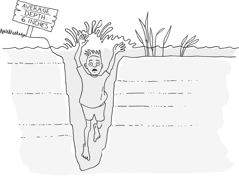
Misled by average depth.
A different statistical measure is more helpful in making realistic estimates: the Annual Failure Rate (AFR) expresses the likelihood that a component will fail in the course of a year. A single disk drive often has an AFR of 1–3 percent. If the AFR is 1 percent, then we would expect roughly one failure each year in every group of 100 disk drives.
However we measure, it’s clear that the overwhelming majority of disk drives don’t fail. We mentioned earlier in this chapter that disk drives are usually the least reliable hardware components. So there’s only a tiny chance that you will ever encounter such a failure on a single disk. This is one reason why people have such trouble with backing up their data: most people get away with not having backups most of the time. It is an unusual experience to have a disk crash on a modern computer. Of course, the rarity of such an experience is little comfort to a person who is nevertheless having that experience, and all the associated disruption (figure 16.10).

“This hardly ever happens.”
Although individual disks may seem incredibly reliable by these measures, they seem almost hopelessly flawed when they are used in very-large-scale computing systems. For example, suppose that we build a disk in which the expected failure rate is only one in a hundred years (3.1 billion seconds)—that might seem like a sufficient level of reliability that we could stop worrying about the issue. But then consider a facility that includes a million of those disks.
Some failure will happen somewhere in that facility about once each hour. Far from being something that we can simply forget about, now the failures of these systems (and dealing with the consequences) has probably become someone’s full-time job. A million disks and their associated failures are not hypothetical extrapolations, they are a present-day reality: Companies like Google and Amazon run multiple data centers, each of which has an enormous array of computing and storage devices. In each of those data centers there is a full-time crew working on replacing and upgrading those devices. When people talk about computing or storing “in a cloud,” it’s useful to keep in mind that there does need to be something real underpinning the “cloudy” abstractions. Those actual underpinnings include not only acres of machines, but also a team of minders.
Suppose now that we’re letting one of those cloud providers take care of all the hardware reliability and availability problems. They may have to do lots of work to provide unstoppable step-taking machinery for us, but that’s no longer our problem; we need to be concerned only about software issues. We take those up in the next chapter.