9 State, Change, and Equality
Although we have considered both the “stepped” nature of digital data and the steps taken by an executing process, we haven’t yet looked very closely at how those ideas interact. We have already seen that a data item can change its value: the “scratch pad” or “tape” of the Turing machine has cells that can be read or written (chapter 3). As we start to consider multiple processes, it’s useful to understand this changeability and its implications more carefully.
As with our examination of names in chapters 4 and 5, some of this examination of changes may seem overdone. But in a similar way, we’ll find that we benefit in later discussions of computer systems and infrastructure. It will be helpful later if we’re careful now about distinctions that may initially seem unimportant.
To start with an everyday example, consider an ordinary coffee cup. Part of what makes a typical coffee cup useful is that it undergoes changes that we can view as different states. A coffee cup typically starts out empty, then it’s filled with coffee, and then it’s partially or wholly emptied by someone drinking the coffee. It may or may not be cleaned before it is refilled with coffee—or if it’s disposable, it will be discarded rather than being cleaned. It usually makes sense to think of it as the same coffee cup throughout the activity: we do not usually think of its identity changing, even though its role in our life may change as it is filled, drained, cleaned. Indeed, there may even be completely different people involved in the filling, emptying, and cleaning (or discarding) stages.
There are many ways we could represent the state of the coffee cup. For example, we may distinguish a few levels like full, partial, or empty. Or we may think of the cup’s state as being clean (ready to be filled) or dirty (ready to be washed). Or we may think of the cup’s state as numbers describing the quantity of coffee contained and the temperature of the coffee there.
To pick another household example, we can consider the slots of a silverware drawer. When all the silverware is out on the table, all of the slots in the drawer are empty. When all of the silverware is freshly washed and put away, the knife slot is full of knives, the fork slot is full of forks, and the spoon slot is full of spoons. In fact, we could even use the silverware slots as a kind of computation mechanism to let us know how many items remain to be put away. Suppose there are eight sets of silverware: eight knives, eight forks, eight spoons. And further suppose that we look in the drawer and see the slots have two knives, five forks, and eight spoons. We can easily figure out that the table or the dishwasher or the sink must have the remaining six knives and three forks. Putting silverware away or taking it out is an analog process (a hand moving continuously through space, with no identifiable discrete “steps” to those hand motions) but we can comfortably view the silverware-in-slots state as being digital: a spoon is either present or absent, and it’s not really interesting or useful to focus on the in-between instants right when the spoon is being taken out or put away.
Stateless vs. Stateful
State complicates behavior. That claim might seem surprising since it wasn’t hard to understand the previous household examples of state. So let’s consider how state adds complexity.
Some circuits or machines have a very simple relationship between inputs and outputs, and identical inputs always produce identical outputs. For example, consider a gadget that’s an adder (not the snake kind), taking two numbers in and producing a single number as a result. An adder that’s given “2” and “3” will always produce the output “5.” There’s no need for any state or history, and no value to adding state. Engineers refer to these as combinational or stateless systems. All you need to know is the combination of inputs to predict the output, because there’s no hidden state to affect that output.
Other circuits or machines depend on some element of previous history to determine outputs. If we see such a machine at an isolated instant of time and without knowledge of the previous history, it’s unwise to try predicting the output. For example, consider the following gadget: each time it’s given two numbers, it adds them both to its previous total. This gadget is not an adder, it’s what a computer scientist would call an accumulator. Like the adder described earlier, this accumulator could also be given “2” and “3” as inputs. But unless we have reason to know its previous total was “0,” there’s no reason to believe the result will be “5.”
Whereas the adder had a simple rule that was applicable for all time, the accumulator has a complex rule that’s contingent on information that we might not know. Engineers refer to systems like the accumulator as sequential or stateful systems. You have to know the sequence or history or the state to predict the output, because the inputs alone are insufficient.
Assignment
When we do simple mathematics, we assume that elements behave in the combinational or stateless way that we described for the adder. If we have a simple algebra problem to solve, we might determine at one step that x = 3. For example, we might have a pair of equations like
2x = 6
y = 3x
Once we’ve learned that first piece of information about x having the value 3 from the first equation, we don’t have to worry that at some later time x might have changed its value to 42. We just go ahead and use the knowledge that x = 3 to determine from the second equation that y = 9.
Indeed, if we are working through a proof and find that there’s some kind of collision of values for a variable (say, we find by one path that x = 3 and by some other path that x = 42) then we’ll declare that there’s a contradiction—and use that contradiction as a basis to reverse some assumption that we made earlier in the proof. For example, if we’re confronted with the following two equations
2x = 6
x = 42
then there’s no solution possible. We would either say that this problem is unsolvable, or we would backtrack to some earlier step of solving the problem to understand whether an earlier error gave rise to the contradiction.
In contrast, a programmer would not be at all surprised to deal with a process in which x has the value 3 at one point and the value 42 at some later point and would see no contradiction or failure. The programmer would simply say that the variable x is mutable; we wouldn’t ordinarily use that word for the changeability of the coffee cup or the silverware drawer, but it’s describing the same characteristic. The mathematical view of variables is correspondingly immutable. In math we might not (yet) know the value for a variable x, but x can have only one value, or else there’s something wrong. In programming, we might see that the same variable x has different values at different times, and that’s OK.
This difference is the root of why state makes it hard to think about processes and their behavior: the same name can have different values at different times in a process’s execution. State means that a particular pairing of a name with a value is not necessarily stable over time. When state is described as an instability of naming, or an instability of values, it becomes a little easier to see why it might not always be a good thing.
Referential Transparency
The very idea of equality has some tricky issues lurking once we introduce mutability into the picture. As we’ve noted, mutability implies that a single name can mean different things at different times. That changeability wrecks a fundamental trick of substituting names for values or vice versa, and means that all kinds of simple statements about the process have to be hedged to the point that they’re essentially useless. Instead of being able to say “x has the value 3” we wind up saying something like “x has the value 3 unless something else changed it, in which case it could be pretty much any value at all”—which in turn seems like a fancy way of saying “we know almost nothing for sure about the value of x.”
It’s handy when a name always has the same value, as in simple mathematics. There is a technical term for this attractive property, and that term is referential transparency—that is, it’s always clear (transparent) what a name refers to. So another way of expressing our concern here is to say that state destroys referential transparency. We can also say that what makes substitution work in our math/algebra examples is that there’s referential transparency. In general, if there is referential transparency, we can say something simple and clear about relationships between names and values; if we don’t have referential transparency, then reasoning about names and values tends to be complex and contingent, often to the point of adding little benefit.
Is State Necessary?
As we start to see the drawbacks of state and how it undercuts referential transparency, we might reasonably ask, Why bother having state? Shouldn’t we get rid of it?
There are two good reasons to have state at least some of the time: expressiveness and physical necessity.
Let’s first consider expressiveness. There are many kinds of activities in the world that are most readily understood or modeled using some kind of mutable state. Our opening example of the coffee cup is one such case. It would be possible to think of the “empty cup” as a completely distinct entity from the “full cup,” and that we somehow switch over from using one to using the other—but it wouldn’t feel very natural as a representation of our everyday experience. If we make a movie of the coffee cup, every frame of the movie has a separate picture of the cup; in a similar fashion, we can break our “stateful” experience of change into a “stateless” form, where change is replaced by multiple instances. But just as it’s more natural to watch a movie than to examine its individual frames, it’s often more natural to deal with state directly, rather than to try to express a stateful behavior in a stateless vocabulary.
In a wide variety of cases, it’s possible to find ways to describe such activities without using mutable state, but those descriptions often seem unnatural and unhelpful to the users who have to judge them. In general, it’s not yet clear whether the advantages of referential transparency are enough to overcome such objections when they are raised. Overall, the rough consensus seems to be that it is a good idea to avoid mutable state when possible but that it’s unwise to outlaw state entirely. It’s nice to have a programming language that allows a state-free style, but not so nice to have a programming language that requires a state-free style.
Now let’s consider physical necessity, and start by returning to a simple program we mentioned when we first started looking at processes (chapter 3). That program prints out “Hi” then pauses a second before doing the exact same thing again, endlessly. When we first mentioned this program, our goal was to point out a simple example of a finite program that corresponds to an infinite process. This program’s endless execution doesn’t require any mutable state: after all, the only activity is printing out the exact same text every time, so the program really doesn’t need to change anything.
But now consider what happens if we modify the program slightly, so that instead of just printing “Hi” repeatedly the program prints “Hi 1” followed by “Hi 2” and then “Hi 3” and so on. There’s nothing about this simple change that requires us to use mutable storage in our program. Although it might seem awkward, we can certainly write the program so that there is a new piece of text created after each previous text has been printed. We can even write the program so that the incrementing counter is simply the next element of an infinite sequence of numbers 1, 2, 3, …. No mutable state is logically necessary in the expression of what this program does.
However, if we run the program and it really has no mutable state used anywhere, it will eventually run out of space. How can we be so sure it will run out of space? Because at each iteration it creates an entirely new text to print—in principle, an infinite number of texts!—and any real step-taking machine has only a finite amount of storage. There’s also something particularly foolish about the way this program runs out of space: it’s full of old numbers and old (already printed) texts. All that leftover data is actually of no value whatsoever for what the program needs to do next.
Of course, there is also a more sensible alternative implementation. We could keep a mutable counter that increments repeatedly through values 1, 2, 3, etc. and then converts that value temporarily into a text for printing, then reuses that space for the next text on the next iteration. It’s not hard to think in terms of a reusable chunk of storage that has “Hi “ at the beginning and then space at the end for a variety of different text representations of numbers like “1” or “2” or “437892” or indeed any other number. But that space-saving approach only works if the counter and text space are mutable, if they can have different values at different points in time.
If we are particularly cunning, we may notice that we could support the appearance of an infinite supply of storage if we were allowed to recycle the old and irrelevant values previously used. Instead of changing the program to use mutable storage, we could change the underlying machine so it looks like it has infinite storage. From the perspective of the program, that’s not mutability—it never sees any value changed. But something is definitely being mutated, because as we watch the machine we can see that a particular storage location holds different values at different times.
Does this issue arise only for infinite programs? No, it’s just easiest to see the problem there. Very similar issues arise whenever a program’s usage of storage might exceed the amount of storage available. Being able to reuse space makes many more computations possible.
Two Kinds of Equal
Whenever there is mutable state, we have to distinguish between (at least) two kinds of “equal.” One kind of equality is an unchanging relationship: two entities that are related by it are always related by it. The other kind of equality is a changeable relationship: two entities that are related by it now might not be related by it later. We’ll call the first relationship “equal-now-and-forever” and the second one “equal-now-but-might-change.”
If we have established that two entities are equal-now-and-forever, then we have referential transparency and we can play substitution games freely. If we have only established that the entities are equal-now-but-might-change, then we don’t have referential transparency. We have to be mindful that we don’t know a lot about how long the two entities will have the same value, unless we know something about how other processes may or may not change them.
If we’re being very careful, we would say that only eternally unchanging entities can ever be “the same as” each other—everything else necessarily changes over time. After all, at a cellular level, you are not exactly the same person you were yesterday. Considered in terms of the interacting atoms and electrons in constant motion, your laptop is not “the same” laptop that it was even a nanosecond ago.
If we do adopt this strict and rather unhelpful perspective, does anything remain equal-now-and-forever? Numeric values don’t change. The value 3 remains equal to every other 3, for example. (We certainly don’t expect the number 3 to suddenly have the value 17.) Similarly, the text “hello” is the same as every other instance of the text “hello.” There’s no risk of it suddenly changing to the string “good-bye.”
Same Object vs. Different Object
The unchanging nature of a value like 3 or “hello” is completely separate from the question of whether some name in the program (like x) has an unchanging value. If we know that a particular name always has the same value, we call it a constant. If we know that a name might not have a value (yet) but can only ever refer to a single value, we can call it a single-assignment variable. In contrast to a constant, a single-assignment variable might not have a value at some point in time; but once it gains a value, that is its value forever, just as if it were a constant with that value. When we looked at simple algebra problems, the mathematical notation behaved like single-assignment variables. If our programming notation only allows names to be constants or single-assignment variables, then that notation will ensure that we always have referential transparency. Such a notation can be called a single-assignment language or a functional language.
But if we don’t have those restrictions, a name might be able to have different values at different times. Whenever that’s true, it doesn’t make much sense to compare using equal-now-and-forever—because anything mutable can’t be equal-now-and-forever to something else, not even itself! The strongest possible form of equality for something mutable is equal-now-but-might-change.
However, saying that we compare mutable state in terms of equal-now-but-might-change isn’t the whole story. In addition, we can (and should!) distinguish between same-object-equal and same-value-equal (see figure 9.1).
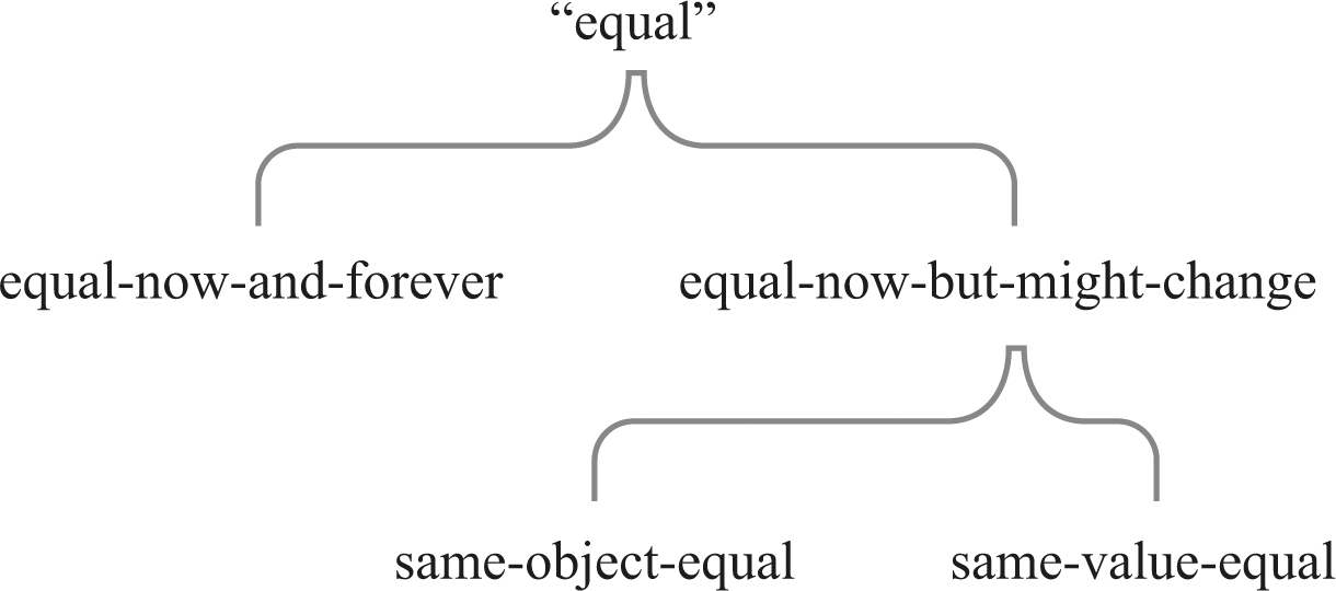
Different kinds of equality.
To understand the difference, let’s consider two names x and y. And let’s say that at the moment both x and y have the value 3. So that means they are same-value-equal (right now!). Finding out that they both have the value 3 doesn’t really give us any information about whether they are same-object-equal.
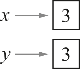
For example, it could be that x and y are both bound eternally to the value 3, as in figure 9.2.
x and y are equal now and forever with the value 3.
That means that x and y are equal-now-and-forever to each other as well as to the value 3. Effectively, x and y are just synonyms for 3.
A seemingly similar situation with very different implications is that x and y are two different names for the exact same mutable cell (which happens to have the value 3 at the moment), as in figure 9.3.

x and y name the same mutable cell containing 3.
The box around the value 3 captures the idea that this is a mutable cell: we can see some later state of the exact same system in which that cell’s value has been changed, as in figure 9.4, where it now has the value 17.
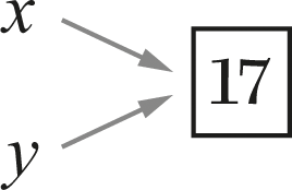
x and y name the same mutable cell, now containing 17.
But yet another configuration that would initially look the same is that x and y could be two completely different things, which just happen to have the exact same value of 3—as in figure 9.5.
x and y name different mutable cells, both containing 3.
In this diagram we have a privileged view in which we can tell whether the names x and y are actually aliases for the same object. We have a means of distinguishing same-object-equal (the two names are actually for the same object) from same-value-equal (the two names happen to have the same value). It’s an important general principle that sharing the same object is quite different from having a separate copy with the same value, and we will pursue that issue further in the next chapter.
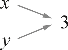
If we don’t have a direct means of determining whether two names refer to the same object, is there any way to tell? Yes, it’s possible to do a kind of experiment: for example, assigning the value 17 to x and then examining the value of y. We will likely conclude that they are not same-object-equal if y still has the value 3, as in figure 9.6.

x and y name different mutable cells with different values.
What if y now also has the value 17? A likely conclusion is that x and y are same-object-equal. However, both of these possible conclusions are actually not as solid or straightforward as you might think: they partly depend on what else might be happening between the actions involved in changing one name’s value and examining the other name’s value. In chapter 11 we will look in more detail at the possibility that other activities are happening in between the steps that we take.
Although at one level state is a familiar everyday concept, we can see that there are a surprising number of subtleties once we examine it closely. On one hand, we seem to live in a stateful universe. It’s easy to find examples where content changes while the identity of the container stays the same—like the coffee cup at the beginning of the chapter. On the other hand, as soon as identity and content can be separated, we have to be very careful about what we mean when we say that two things are “the same” or “equal.” Simple reasoning seems to depend on avoiding state, while realistic implementation seems to depend on using state. We might paraphrase a famous saying of Erasmus: State, can’t live with it, can’t live without it.