Thus far it has been assumed that spacetime is the flat spacetime of Minkowski space. If a “particle” is real, one would expect it to exist near a massive body whether the spacetime is curved or not. In addition, one would expect that the coordinate frame used should not affect the existence of the particle nor should it generate particles. The Unruh effect and Hawking radiation, discussed below, show that this assumption could be incorrect.1
Vacuum Fluctuations
As was discussed earlier, both Schwinger and Pauli cast doubt on the reality of vacuum fluctuations. In Schwinger’s source theory, the vacuum is “the state of zero energy, zero momentum, zero angular momentum, zero charge, zero whatever,” and Pauli who stated that “it is quite impossible to decide whether the field fluctuations are already present in empty space or only created by the test bodies” and as late as 1946, he is quoted as saying that “zero-point energy has no physical reality.”
There is some ambiguity about the term “vacuum fluctuations” and “zero-point energy” in the literature. If one is discussing the lowestenergy or ground state of some quantum mechanical system, the uncertainty principle tells us that the Hamiltonian must contain the term ℏω/2.
If an electric, magnetic or vector potential field is present in the vacuum, the vacuum expectation of its field operator will vanish, but the expectation of the square of the field operators will not, which implies there are what are often called vacuum fluctuations of the field. In quantum field theory, each point in space has this zero-point energy associated with it, thus leading to infinite energy in any finite volume.
Zero-point energy, and fluctuations associated with it, may be eliminated by normal (Wick) ordering. But expectation values of normalordered operators vanish only for the free theory. In the interaction picture of quantum field theory, normal ordering eradicates Feynman diagrams with internal lines that begin and end on the same internal vertex. Higher order Feynman diagrams can be eliminated by what is known as complete normal ordering.2
It is often said that even the vacuum empty of all fields still retains the zero-point energy, whose average energy vanishes. What is left are the vacuum fluctuations of the so-called virtual particles that satisfy ΔEΔt ≥ ℏ so that energy can be taken from the vacuum to allow particles to appear for very short times. These are the type of vacuum fluctuations that apply to the Unruh and Hawking effects and whose reality Schwinger and Pauli doubted.
More recently, Jaffe3 has pointed out that the Casimir effect, often cited as the proof that vacuum fluctuations are real, and its experimental confirmation does not establish the reality of zero-point fluctuations. He points out that vacuum-to-vacuum Feynman graphs, that essentially define the zero-point energy, are not involved in the calculation of the Casimir force, which only involves graphs with external lines. In conclusion, he states that there is “no known phenomenon, including the Casimir effect, [that] demonstrates that zero point energies are ‘real’.”
Casimir calculated the attractive force between two uncharged parallel conducting plates due to the quantum electromagnetic zero-point energy of the normal modes between the plates. But whether the force is attractive or repulsive depends on the geometry of the uncharged conductor.4
A discussion of how the vacuum is defined and the relation of vacuum fluctuations to the Casimir effect and the cosmological constant problem are contained in Appendix C.
The Unruh Effect
The Unruh or Davies–Unruh effect occurs for a uniformly accelerated detector in a vacuum that would measure a temperature given by T = ℏa/2πckB, where a is the local acceleration and kB is the Boltzmann constant. This temperature has the same form as the Hawking temperature of a black hole TH = ℏg/2πckB, where g is the surface gravity of the hole. In the case of the hole, there is spontaneous particle creation. Although the two effects are mathematically and physically distinct, they are superficially related by the equivalence principle between acceleration and gravitation.
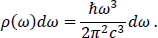
The electromagnetic zero-point fluctuation of the vacuum may be regarded as a propagating electromagnetic field with a spectral energy density5
There has been some debate over whether this field should be regarded as real or virtual. The evidence given to support the reality of the various contributions to the vacuum energy is the Casimir effect, which is a consequence of the lowest order vacuum fluctuations, and higher order effects like the Lamb shift. But there are alternative explanations. The Casimir effect could result from fluctuations associated with the constituents of the plates rather than vacuum fluctuations. Schwinger’s source theory takes this point of view and avoids vacuum fluctuations in both the Casimir and higher order QED effects. And Pauli’s opinion was quoted above.
The spectral energy density given above is Lorentz invariant, but in a uniformly accelerated reference frame with proper acceleration a one finds a pseudo-Planckian spectrum with a radiation temperature T = ℏa/2πckB, the same as that for the Unruh effect. In this frame, the spectral energy density has the form
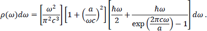
Notice that at high frequencies this reduces to the previous expression. The Unruh effect is thus due to the lower frequencies.6
The two above spectral energy densities tell us that the vacuum state is not the same in an unaccelerated inertial frame and an accelerated one. But general relativity tells that the coordinates used are arbitrary and have no geometrical or physical meaning. As put by Misner, Thorne and Wheeler in their book Gravitation: “The laws of physics, written in component form, change on passage from flat spacetime to curved spacetime by a mere replacement of all commas by semicolons,” where the comma represents ordinary partial differentiation and the semicolon covariant differentiation. The laws of classical physics are local in nature and the comma-goes-to-semicolon rule is directly related to the equivalence principle. If one believes vacuum fluctuations are real, then one must accept that not all coordinate systems are physically equivalent in quantum mechanics.
In spite of the enormous literature on the Unruh effect, this has been unpalatable for many and some maintain that the effect does not exist.7 I will not go through the technical details of the argument, but simply give an outline.
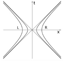
The coordinates of a reference frame in Minkowski space accelerating with a constant proper acceleration are, in the context here, often called Rindler coordinates. The figure below shows the left (L) and right (R) Rindler wedges in Minkowski space. The hyperbolic paths of two objects undergoing constant proper acceleration are shown. The closer the hyperbola is to the origin, the greater the acceleration. The light cone represents the event horizons bordering the part of Minkowski space accessible to “Rindler observers”. The interior of the R wedge, an incomplete manifold, is called Rindler space.
Narozhny et al.,8 showed that one can attach physical meaning to the Unruh method of quantization only in the double Rindler wedge consisting of L and R, with their regions not being causally connected. The Unruh construction requires that boundary conditions be imposed on the origin (or two-dimensional plane in the case of (3 + 1) dimensional spacetime). These boundary conditions constitute a topological obstacle that disallows any correlation between particles in the L and R wedges. This means that the averaging over quantum field states in one wedge cannot lead to thermalization of states in the other wedge. A free quantum field in Minkowski space cannot be decomposed into two noninteracting fields, one in the L wedge and the other in the R wedge.
At this point, I will quote the very well supported conclusion of Narozhny et al.: “Hence, considerations of the Unruh problem, both in the standard and algebraic formulations of quantum field theory as of now do not give convincing arguments in favor of a universal thermal response of detectors uniformly accelerated in Minkowski space.” Given the intense controversy over the issue, it is worth looking at the Acknowledgements list in this paper.
Hawking Radiation
Although the Unruh and Hawking effects are generally thought to be mathematically and physically distinct, there is a good argument which shows that their relationship through the equivalence principle is closer than one might think.
One often finds Hawking radiation described as the thermal radiation predicted to be spontaneously emitted by black holes, which arises from vacuum fluctuations of particle and antiparticle pairs. One of the particles of the pair is absorbed by the horizon and the other is identified with the Hawking radiation. However, the best way to understand Hawking radiation is to consult Hawking’s very clear original 1975 paper.9
Numerous authors have discussed the fact that the vacuum and particle states arising in the canonical quantization of the free scalar field depend upon the coordinate system within which the Klein–Gordon equation is solved. The procedure used is to solve the Klein–Gordon equation for the normal modes appropriate for a given curvilinear coordinate system, and relate these to the plane-wave mode solutions in rectilinear Minkowski coordinates via a Bogoliubov transformation.10 If the coefficient in this transformation corresponding to an admixture of positive and negative frequency modes is non-zero, particles will be present. The mixing of positive and negative frequency modes also implies that the vacuum states will differ. What follows is a brief introduction to these concepts.
A distinction between positive and negative frequency solutions to a general spacetime is possible only if the spacetime possesses a global Killing vector field. This will be assumed to be the case. The generalization of the Klein–Gordon equation to a general spacetime is

where

and ∇ is the covariant derivative. Since the existence of a global time-like Killing vector K is assumed, the normal mode solutions of Eq. (B.2) may be chosen to satisfy

Where  is the Lie derivative with respect to K. The presence of a Killing vector means that

If the coordinate system is chosen such that only the non-zero component of the Killing vector is a unit vector along x0, then Eq. (B.3) can be written as

and Eq. (B.1) can be solved by separation of variables by the substitution

If ψ1 and ψ2 are complex solutions of Eq. (B.1) and Σ is any complete Cauchy hypersurface for this equation, an inner product can be defined as
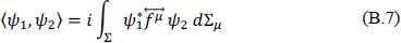
where,

and dΣµ is the outwardly directed surface element of Σ. The value of 〈ψ1, ψ2〉 is independent of Σ. The arrows above the partial derivatives denote whether the derivative is acting to the left or the right.
The field may then be quantized by defining a field operator11
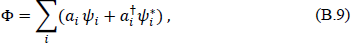
its conjugate momentum Πµ = g1/2gµν∂xνΦ, and imposing the usual commutation relations,
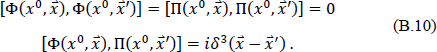
Using the definition of Πµ and Eq. (B.9) gives, when combined with Eq. (B.10), the commutation relations for the annihilation and creation operators a and a†,

Note that a and a† are operators with no time or space dependence, and ψi and  correspond respectively to positive and negative frequency solutions.
Consider now a second set of modes  , which in the present context arise from solving the Klein–Gordon equation, (B.1), in some flatspace coordinate system other than rectangular Minkowski coordinates. The new modes can be expanded in terms of the old modes of Eq. (B.9) as
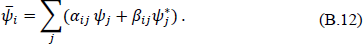
The inner product, Eq. (B.7), can be used to determine the αij and βij as

If the field operator Φ is to be expanded in terms of the new modes as
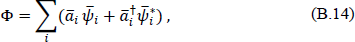
the new creation and destruction operators āi and  must be related to the old by

These equations are known as a Bogoliubov transformation of the operators a and a†.
For Eqs. (B.9) and (B.14) to be consistent, and if ā and ā† are to satisfy the same commutation relations as a and a†, the Bogoliubov coefficients introduced above must satisfy
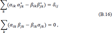
or, in equivalent but somewhat redundant matrix notation,
where the tilde corresponds to matrix transposition.
One can now define the particle number operator, which is the sum of the particle-number operator for each of the states. It is possible to find a common set of eigenstates for these commuting operators, each of which are fully characterized by specifying the particle numbers. In this way, one can form the basis of the particle number representation of the Hilbert space, sometimes called the Fock space.
However, since there are two vacuum states, |0⟩ and  , where ai|0⟩ = 0 and
  for all i, two Fock spaces are necessary and they will differ if βij ≠ 0. This can be seen by direct computation of the matrix element
  :
:

which can be written, by summing over i, as the number operator,  ,
,

is interpreted as the average number of -mode particles in the vacuum state |0⟩. Note that if diverges, the two vacuum states |0⟩ and are not related by a unitary transformation.
The Underlying Physics of Hawking Radiation
Over twenty-five years ago Punsly12 proposed that a global quantum field theory such that in a Schwarzschild background space when restricted to any point in that space is consistent with the field theory found by a freely falling observer at that point. This can be expanded to small regions of spacetime much less than the radius of curvature.
The equivalence principle demands that the field theory found by a freely falling observer be locally the same as that in flat spacetime. Punsly’s approach predicts that an isolated black hole will emit thermal radiation that can be identified with Hawking radiation. He showed that the renormalized stress-energy tensor is a measure of the change in the energy of the zero-point oscillations of the field theory as formulated by a freely falling observer; an observer at infinity sees the zero-point energy decrease as this observer approaches the black hole horizon. The freely falling observer sees no particles in the local vacuum; i.e., Hawking radiation does not exist for a freely falling observer.
• • •
What is shown above is that both the Unruh effect and Hawking radiation depend on the reality of vacuum fluctuations as defined in the first part of this Appendix. Because there is as yet no truly compelling evidence that these fluctuations actually exist, the Unruh effect and Hawking radiation may well be illusory.
Charge, Spacetime Geometry, and Effective Mass13
When one thinks of solutions to the Einstein gravitational field equations, it is often thought that the solutions only have a positive curvature of spacetime associated with them. But this is not always true even for spherically symmetric non-rotating solutions or those having angular momentum. This section shows how negative curvature arises due to electric charge.
Charge, like mass in Newtonian mechanics, is an irreducible element of electromagnetic theory that must be introduced ab initio. Its origin is not really a part of the theory. Fields are then defined in terms of forces on either mass — as in the case of Newtonian mechanics, or charges in the case of electromagnetism. General Relativity changed our way of thinking about the gravitational field by replacing the concept of a force field with the curvature of spacetime. Mass, however, remained an irreducible element. It is shown here that the Reissner–Nordström solution to the Einstein field equations tells us that charge, like mass, has a unique spacetime signature.
The Reissner–Nordström solution is the unique, asymptotically flat, and static solution to the spherically symmetric Einstein–Maxwell field equations. Its accepted interpretation is that of a charged mass characterized by two parameters, the mass M and the charge q. While this solution14 has been known since 1916, there still remains a good deal to be learned from it about the nature of charge and its effect on spacetime.
It will be shown here that if the source of the field is the singularity of the vacuum Reissner–Nordström solution, only the Schwarzshild mass is seen at infinity, with the charge and its electric field making no contribution. In particular, if the charge alone is the source of the field, the effective mass seen at infinity vanishes. This is not the case when the source of the field is a “realistic” source characterized by a mass and proper charge density. It will also be seen that the presence of charge results in a negative curvature of spacetime.
The Reissner–Nordström solution is given by

where m = GM/c2 and Q = (G1/2/c2)q. The Reissner–Nordström metric reduces to that of Schwarzschild for the case where Q = 0. Notice that this metric takes the Minkowski form when r = Q2/2m.
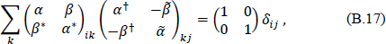
If Q2 ≤ m2 , this solution has two apparently singular surfaces located at 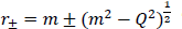 . These are coordinate singularities that may be removed by choosing suitable coordinates and extending the manifold. If Q2 = m2, these surfaces coalesce into a single surface located at r = m, and if Q2 > m2 the metric is non-singular everywhere except for the origin. These singular surfaces play no role in what follows. An extensive discussion of the vacuum Reissner–Nordström and Schwarzschild solutions, along with their Penrose diagrams was given by Hawking and Ellis.15
Most applications of the Reissner–Nordström solution would be outside a body responsible for the charge and mass. Here it is the vacuum solution to the field equations, considered to be valid for all values of r, that is of interest.
Like the vacuum Schwarzschild solution, the Reissner–Nordström vacuum solution has an irremovable singularity (in the sense that it is not coordinate dependent) at the origin representing the source of the field. In what follows, only the Reissner–Nordström solution having this singularity as a source of the field will be considered.
The interesting thing about the singularity is that it is time-like so that clocks near the singularity run faster than those at infinity. It is also known that the singularity of the Reissner–Nordström solution is repulsive in that time-like geodesics will not reach the singularity.
Curvature in the Reissner–Nordström Solution
If one computes the Gaussian curvature associated with the Schwarzschild solution, it is readily seen that the curvature vanishes. Higher order scalars, such as the Kretschmann scalar given by K = RαβγδRαβγδ, do not vanish, but their interpretation is problematic.16 Of course, the curvature of spacetime around a Schwarzschild black hole does not vanish since the curvature tensor does not vanish. More important for the present discussion is that a simple way to determine the sign of the curvature is well known.
Consider first the Schwarzschild solution. Draw a circle on the equatorial plane where θ = π/2 is centered on the origin. The circumference of this circle is 2πr. The proper radius from the origin to the circle is given by

Consequently, the ratio of the circumference of the circle to the proper radius is less than or equal to 2π. This tells us that the space is positively curved. Now consider a negative mass. The inequality sign in Eq. (B.21) reverses so that the ratio of the circumference of a circle to its proper radius is greater than 2π, telling us that the space surrounding a negative mass has a negative curvature.
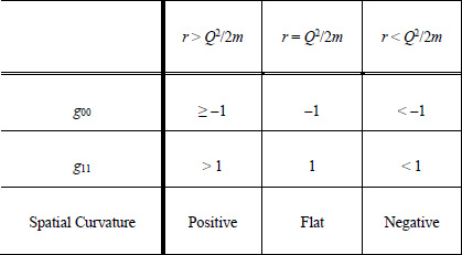
The case of the Reissner–Nordström solution is more interesting. Setting
and using the above method of determining the spatial curvature gives the results shown in Table 1. For r < Q2/2m, one has a negatively curved spacetime, which is embedded in a positively curved spacetime with a (2 + 1) dimensional boundary having the Minkowski form between them. In the region between the time-like singularity at the origin and the (2 + 1) dimensional hypersurface, the spacetime is negatively curved independent of the sign of the charge. This implies that charge manifests itself as a negative curvature — just as mass causes a positive curvature.
Table B.1. The metric coefficients g00 and g11 for different ranges of r, and the sign of the spatial curvature in these regions.
That charge effectively acts as a negative mass can also be seen from the equations governing the motion of a test particle near a Reissner–Nordström singularity. For an uncharged particle falling inward towards the singularity the radial acceleration is,17
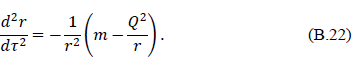
The gravitational field that affects the test particle varies with distance from the singularity and becomes repulsive when the effective mass 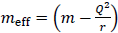 becomes negative at r < Q2/m. Neutral matter falling into the singularity would therefore ultimately accumulate on the (2 + 1)-dimensional spherical hypersurface where meff = 0.
Thus, by means of very straight-forward considerations, the Reissner–Nordström solution leads to the conclusion that charge — of either sign — causes a negative curvature of spacetime.
The Electric Field
This section is devoted to a general relativistic calculation of the effective mass of the vacuum Reissner–Nordström solution: first, of that contained within the interior of a spherical surface of radius R, centered on the singularity — and designated  ; and second, the effective mass of the electric field alone outside that surface — designated
  . The key references for what follows are Synge,18 and Gautreau and Hoffman.19
Synge gives the following Stokes relation20 for a three-dimensional volume, v3, bounded by a closed two-surface v2:
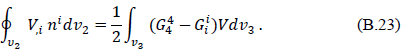
Here, dv2 and dv3 are the invariant elements of area and volume, G is the Einstein tensor, and V is defined by the line element

which, at infinity, is assumed to take the form of the Minkowski metric. ni is the outward unit normal to the surface v2. Einstein’s equations, Gµv = −kTµν, with k = 8π, allow Eq. (B.23) to be written as
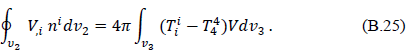
The integral on the right-hand side of this equation corresponds to the total effective mass enclosed by the surface v2. This is known as Whittaker’s theorem.21 Thus,

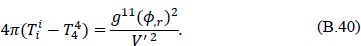
Note that the effective mass, as defined by Eqs. (B.25) and (B.26), depends only on the energy-momentum tensor and the g00 component of the metric. Choose a spherical surface of radius R with the Reissner–Nordström singularity at the origin. From Eq. (B.20), V is given on the surface as
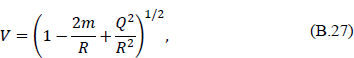
dv2 = R2 sin θdθdφ and ni = (V, 0, 0). Substituting into Eq. (B.26) gives the result quoted above [ just after Eq. (B.22)] for meff at a distance R from the singularity
For asymptotically flat spacetimes, global quantities such as the total energy can be defined as surface integrals in the asymptotic region. This is the basis for the definition of the ADM energy (or mass).22 What will be shown here is that for R ≠ ∞, the sum of the effective mass within the surface v2 and that exterior to v2 is the Schwarzschild mass. This is true for the vacuum solution being considered here, not necessarily for realistic sources such as those considered by Cohen and Gautreau.
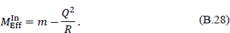
Whittaker’s theorem allows the effective mass enclosed by the surface v2, which is composed of the mass located at the origin and that corresponding to the electric field within v2, to be written as in Eq. (B.28).
One can also compute the effective mass exterior to the surface v2. There, the only energy density to be found is that associated with the electric field. By summing the effective mass found in the volumes both interior and exterior to v2, one obtains the effective mass enclosed by the surface at infinity; that is, the ADM mass. Given that global quantities defined by surface integrals in the asymptotic region cannot generally be written as volume integrals over the interior region, this is a somewhat surprising result.
How to use the relation of Eq. (B.25) to compute the electric field energy in the volume exterior to the spherical surface of radius R centered on the singularity can be understood by referring to Fig. B.1. The volume of interest is  exterior to the surface v2. It has two boundary components, the “surface at infinity” and v2 itself.
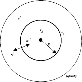
Fig. B.1. The Reissner–Nordström singularity is located at the center of the spherical surface v2 of radius R enclosing the volume v3. The outward pointing unit normal to v2 is ni. The surface enclosing the volume is composed of the point at infinity and v2. The outwardly pointing unit normal to v2, when acting as a boundary component of , is n′i.
Since the surface integral at infinity vanishes, Eq. (B.25) for the volume may be written as
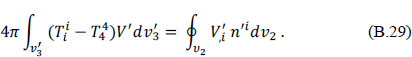
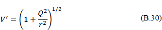
The V in Eq. (B.25) has been changed to V′ in Eq. (B.29). The reason for this is that the energy-momentum tensor in the volume must be restricted to the contribution from only the electric field since no masses exist in . The way to do this is to recognize that the Reissner–Nordström solution remains a solution to the Einstein field equations even when the mass m is set equal to zero. The resulting metric is that for a massless point charge, which — as discussed above — has a negative curvature and is repulsive. The energy-momentum tensor for the electric field nonetheless has a positive energy density. The V′ that should be used in Eq. (10) is therefore that from the metric for a massless point charge; i.e.,
Note that r takes the fixed value R when computing the surface integral.
Because ni = −n′i, the effective mass contained in the volume exterior to v2 is

can be evaluated by simply using the second integral in Eq. (B.31), which was already evaluated for V above. Taking account of the orientation of the surface and the substitution of V′, the result is

Combined with Eq. (B.29), this results in

What this tells us is that the “negative mass” associated with the charge Q [see Eq. (B.28)] is exactly compensated by the effective mass contained in the electric field present in the volume exterior to the surface r = R. If the radius r = R → ∞, the effective mass contained within the surface at infinity is m, the Schwarzschild or equivalently, the ADM mass.
One can also obtain the result given in Eq. (B.33) by directly evaluating the last integral on the right-hand side of Eq. (B.31). This will be done here for the sake of completeness as well as a confirmation of Eq. (B.32) above. To begin with, an identity relating the energymomentum tensor  of the electric field to the scalar potential is needed.
If the energy-momentum tensor

where
is restricted to the case where only electric fields are present, so that

then it is readily shown that

Equations (B.36) allow the energy-momentum tensor to be written as
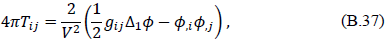
where Δ1 is a differential parameter of the first order defined23 by

The needed identity may now be obtained from Eq. (B.37) as

which, for spherical coordinates, may be written as
The total effective mass inside the three-volume d is then
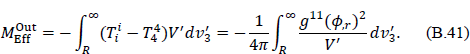
Substitution of V′ from Eq. (B.30), along with  , ϕ = Q/r, and
 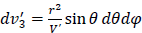 , yields

As expected, this is the same result as that given in Eq. (B.32).
Summary
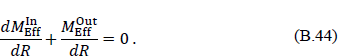
The above results may then be summarized as in Eq. (B.33)
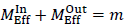
independent of the radius R. What this says is that the amount of “negative mass” due to the term −Q2/R in Eq. (B.28) is exactly compensated by the amount of “positive mass” contained in the region r > R. For R infinite, is the Schwarzschild mass; and if R < ∞, is less than the Schwarzschild mass.
In their 1979 paper, Cohen and Gautreau noted that: “As R decreases, MT [here equal to ] also decreases because the electric field energy inside a sphere of radius R decreases.” And, one might add, as R decreases, the field energy exterior to R increases. This is equivalent to

so that
While charge of either sign causes a negative curvature of spacetime, the Einstein–Maxwell system of equations does not allow different geometric representations for positive and negative charges. This is a direct result of the fact that the sources of the Einstein–Maxwell system are embodied in the energy-momentum tensor, which depends only on the (non-gravitational) energy density — which is why charge enters as Q2 above. Thus, a full geometrization of charge does not appear to be possible within the framework of the Einstein–Maxwell equations.
As mentioned earlier, no “realistic” sources for the Reissner–Nordström metric are considered in this paper. Realistic sources raise many interesting questions, among them are: Can a lone, charged black hole actually exist? If so, how can global charge neutrality be maintained?
• • •
The above applied to the vacuum Reissner–Nordström metric, but the work can be extended to charged rotating vacuum solutions of the Einstein field equations, and in particular, to the Kerr–Newman solution.24
The Kerr–Newman solution in generalized Eddington coordinates,25 which are convenient for this approach, is given by
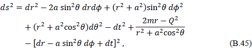
where the symbols have their conventional meanings.
It was pointed out above that for the Reissner–Nordström solution the metric takes the Minkowski form when r = Q2/2m. Interestingly enough, the same thing occurs in the Kerr–Newman metric except that now r has a different meaning with surfaces of constant r corresponding to confocal ellipsoids satisfying
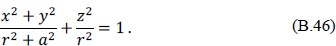
It will be seen, however, that unlike the Reissner–Nordström solution, where it was possible to show that for r < Q2/2m the curvature was negative, the case of the Kerr–Newman solution is more complex. An indication of this is given in Fig. B.2.

Fig. B.2. The ratio of the circumference to the radius R in the equatorial plane of the Kerr–Newman solution in Eddington coordinates. The ring singularity of the Kerr–Newman metric is at r = 0. The portion of the curve above the line C/R = 2π corresponds to a negative curvature and that below to positive curvature. C/R = 0 at r ~ 0.404698 where gϕϕ = 0, and crosses the line C/R = 2π at r = Q2/2m, which for the value of the parameters used here, a = m = Q = 1, is 0.5.
Here the negative contribution of rotation to the effective mass for the Kerr–Newman metric has been excluded. The “negative mass” due to charge has properties very similar to that of the Reissner–Nordström metric. Both take the Minkowski form at r = Q2/2m, even though the meaning of r is different for the two metrics; the effective mass interior to this surface is −m in both cases; and both have an effective mass of m at infinity. In addition, the effective mass for both metrics satisfies, for any surface defined by r = constant (again for either definition of r), the relation

Thus, the positive effective mass of the electric field exterior to the surface exactly compensates for the “negative mass” associated with the charge located within the surface.
____________________________________
1 A key reference for the Unruh and Hawking effects is: R. M. Wald, Quantum Field Theory in Curved Spacetime and Black Hole Thermodynamics (The University of Chicago Press, Chicago, 1994). Clear derivations are also given in: P. W. Milonni, The Quantum Vacuum (Academic Press, Inc., Boston, 1994).
2 J. Ellis, N. E. Mavromatos, and D. P. Skliros, “Complete normal ordering 1: Foundations,” Nucl. Phys. B 909 (2016), 840–879.
3 R. L. Jaffe, “Casimir effect and the quantum vacuum,” Phys. Rev. D 72 (2005), 021301; arxiv:hep-th/0503158 (2005).
4 T. H. Boyer, Phys. Rev. 174 (1968), 1764. See also: W. Lukosz, Physica 56 (1971), 109; Z. Physik 258 (1973), 99.
5 T. H. Boyer, Phys. Rev. 182, 1374; P. W. Milonni, The Quantum Vacuum (Academic Press, Inc., Boston, 1994), p. 49.
6 See B. Haisch, A. Rueda, and H. E. Puthoff, “Inertia as a zero-point-field Lorentz force, Phys. Rev. A 49 (1994), 678–694.
7 See, for example, V. A. Belinskii et al., JETP Lett. 65 (25 June 1997), 902.
8 Narozhny et al., Phys. Rev. D 65 (2001), 025004.
9 S. Hawking, Commun. Math. Phys. 43 (1975), 199–220.
10 These transformations were introduced by Bogoliubov in the context of solid-state physics (Zh. ETF 34 (1958), 58 [JETP 7 (1958), 51]).
11 The symbol * is the complex conjugate and † is the adjoint or Hermitian conjugate.
12 B. Punsly, “Black-hole evaporation and the equivalence principle,” Phys. Rev. D 46 (1992), 1288–1311.
13 This section originally appeared in: G. E. Marsh, Found. Phys. 38 (2008), 293–300.
14 H. Reissner, “Über die eigengravitation des elektrischen feldes nach der Einstein’schen Theorie,” Ann. Physik 50 (1916), 106–120; G. Nordström, “On the energy of the gravitational field in Einstein’s theory,” Verhandl. Koninkl. Ned. Akad. Wetenschap., Afdel. Natuurk., Amsterdam 26 (1918), 1201–1208.
15 S. W. Hawking and G. F. R. Ellis, The Large Scale Structure of Space-Time (Cambridge University Press, Cambridge, 1973), pp. 156–161.
16 The divergence of the Kretschmann scalar as r → 0 indicates a real — as opposed to a coordinate dependent — singularity. It has been proposed that the Kretschmann scalar be called “the spacetime curvature” of a black hole; see: R. C. Henry, “Kretschmann scalar for a Kerr–Neuman Black Hole”, Astrophys. J. 535 (2000), 350–353.
17 V. de la Cruz and W. Israel, “Gravitational bounce,” Nuovo Cimento 51 (1967), 744; J. M. Cohen and D. G. Gautreau, “Naked singularities, event horizon, and charged particles,” Phys. Rev. D 19 (1979), 2273–2279; W. A. Hiscock, “On the topology of charged spherical collapse,” J. Math. Phys. 22 (1981), 215; F. de Felice and C. J. S. Clarke, Relativity on Curved Manifolds (Cambridge University Press, Cambridge, 1992), pp. 369–372.
18 J. L. Synge, Relativity: The General Theory (North-Holland Publishing Company, Amsterdam, 1966), Ch. VII, §5 and Ch. X, §4.
19 R. Gautreau and R. B. Hoffman, “The structure of the sources of Weyl-type electrovac fields in general relativity,” Nuovo Cimento 16 (1973), 162–171.
20 Greek indices take the values 1, 2, 3, 4 and Latin indices 1, 2, 3. To avoid unnecessary confusion, the notation used here is generally consistent with that found in the relevant literature.
21 E. T. Whittaker, “On Gauss’ theorem and the concept of mass in general relativity,” Proc. Roy. Soc. London A149 (1935), 384.
22 R. Arnowitt, S. Deser, and C. W. Misner, “The dynamics of general relativity,” contained in L. Witten (ed.), Gravitation: An Introduction to Current Research (John Wiley & Sons, Inc., New York, 1962), pp. 227–265.
23 L. P. Eisenhart, Riemannian Geometry (Princeton University Press, Princeton, 1997), p. 41.
24 G. E. Marsh, “Charge geometry and effective mass in the Kerr-Newman solution to the Einstein field equations,” Found. Phys. 38 (2008) 959–968.
25 An excellent discussion of these coordinates and their interpretation can be found in R. H. Boyer and R. W. Lindquist, “Maximal analytic extension of the Kerr metric,” J. Math. Phys. 8 (1967), 265–281.