Appendix F
Lauter Tun Design for Continuous Sparging
Continuous sparging is all about understanding steady state flow. We need to understand how the sparge water is going to flow through the grain bed so we can predict where the grain will be rinsed of sugar and where it won’t. Before I lead you through all the theory and explanations, let me cut to the chase and tell you how it works best:
- • A false bottom works best, but a large multi-pipe manifold works almost as well.
- • Regulate the flow with a valve to achieve a slow flow rate—about 1 qt. or 1 L per minute—to prevent compaction of the grain bed and channeling.
- • Maintain an inch (couple of centimeters) of water over the grain bed during the lauter to ensure fluidity and free flow.
To explain why false bottoms work best, I have to turn to fluid dynamics and some mathematical models that a friend put together for me. I spent a year conducting fluid flow experiments with ground-up corncobs and food coloring in an aquarium in order to understand how slotted pipes worked under continuous sparging. Those experiments demonstrated that the flow converged to the pipe and that all points along a slotted pipe drained at the same rate, regardless of distance to the drain (see fig. F.1).
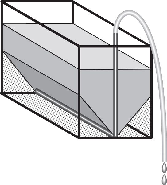
Figure F.1. Depiction of fluid flow to a single pipe. The flow converges, leaving unsparged zones in the corners.
The goal in the continuous sparging process is to rinse all of the grain particles in the tun of all their sugar. To do this we need to focus on two things:
- • Keep the grain bed completely saturated with water.
- • Make sure that the fluid flow through the grain bed to the drain is slow and uniform.
By keeping the grain bed covered with at least an inch of water, the grain bed is in a fluid state and not subject to compaction by gravity. Each particle is free to move and the liquid is free to move around it. Settling of the grain bed due to loss of fluidity leads to preferential flow and poor extraction.
Continuous sparging depends on being able to rinse the sugars from the grain, and a big part of this process is diffusion. If you rinse quickly you will end up with mostly sparge water in your boiler, because the sugar won’t have time to diffuse into the sparge water as it flows past.
Fluid Mechanics
To extract the wort from all regions of the grain bed, there must be fluid flow from all regions to the drain. In a perfect world, the wort would separate easily from the grain and we could simply drain the grain bed and be done. However, it is not a perfect world, and we must rinse, or sparge, the grain bed to get most of the sugars, and some sugar is still left behind. If some regions of the grain bed are far from the drain, and experience only 50% of the sparge flow, then only 50% of the wort from those regions will make it to the drain. Fluid mechanics allows us to model the flow rates for all regions of the grain bed and determine how well a grain bed is rinsed. These differences can be quantified, enabling us to compare different lauter tun configurations.
To illustrate, let’s look at a cross section of a 10-inch wide by 8-inch deep lauter tun that uses a single pipe manifold (fig. F.2). For every unit volume of water that rinses the grain bed, grain at the top of the grain bed will experience “unit” flow, that is to say, 100% flow. As the flow moves deeper into the grain bed, it must converge to the single drain. This means that the region immediately above the drain can experience ten times the unit flow, while a region off to the side will only experience one-tenth of unit flow. The vector flow plot for a lauter tun of the same size that uses two pipes demonstrates the same behavior (fig. F.3), although the convergence effect is less. Figure F.4 shows the flow rate distribution for the single pipe manifold lauter tun. For purposes of illustration, unit flow (the big white upper area) is drawn within the bounds of ±10% of actual unit flow, and lines for 50%, 90%, 110%, and 200% of unit flow are shown. Figures F.2 and F.4 convey the same idea, but figure F.4 lets us quantify the percentages of flow for this grain bed. The histogram (fig. F.5) constructed from this data summarizes the flow distribution and we can use the histogram to measure two aspects of lautering performance—efficiency and uniformity. For comparison, flow distribution and associated histogram for a full-sized false bottom are illustrated in figures F.6 and F.7. The differences will be explored more fully in the next couple of sections as we look at the concepts of lauter efficiency and uniformity.
Figure F.2. Lauter Flow Vectors
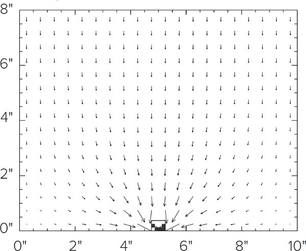
Figure F.3. Lauter Flow Vectors
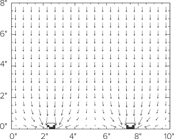
Figure F.2 and F.3. These diagrams show the flow vectors in a lauter tun consisting of a single pipe (F.2) and double pipes (F.3). The size of the arrows indicates the relative speed of flow. Note how the flows converge to the pipes, leaving low flow areas in the corners. This same behavior has been observed when flowing food coloring dye through a grain bed in a glass aquarium.
Single-pipe flow rates
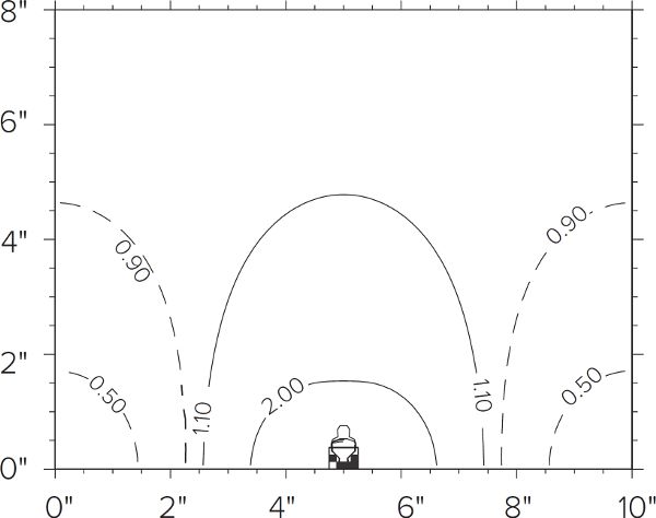
Figure F.4. Flow rate distribution for the same single-pipe lauter tun shown in figure F.2. Darcy’s Law allows us to quantify the flow velocity at any point within the lauter tun. The lines show the boundaries for 50%, 90%, 110%, and 200% of unit flow velocity. The area above the 0.90 and 1.10 flow lines is a region of 100% uniform flow.
Single-pipe histogram
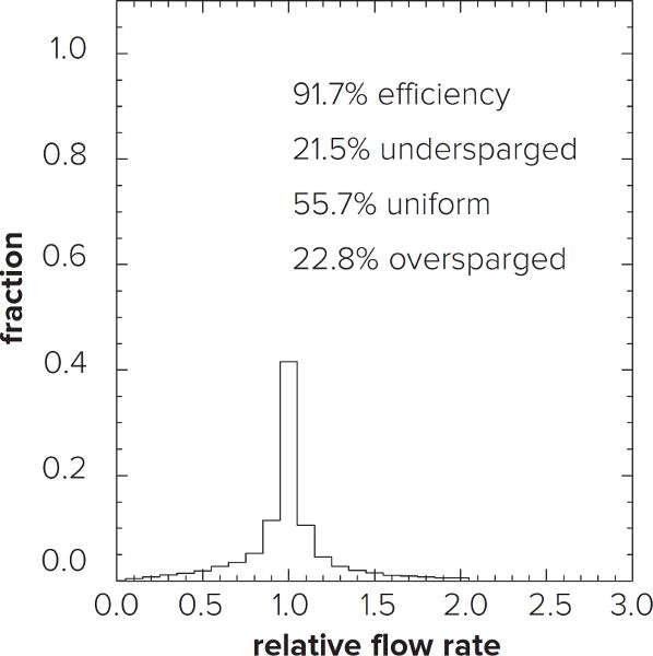
Figure F.5. Histogram showing the relative amounts of different percentages of unit flow as described by figure F.4.
False bottom flow rates
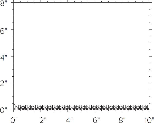
Figure F.6. Flow rate distribution for a lauter tun with a full-sized false bottom. As in figure F.4, the lines show the boundaries for 50%, 90%, 110%, and 200% of unit flow, but the convergence zone is so small that you can’t pick them out. This false bottom model represents ⅛" holes on ¼" centers.
False bottom histogram
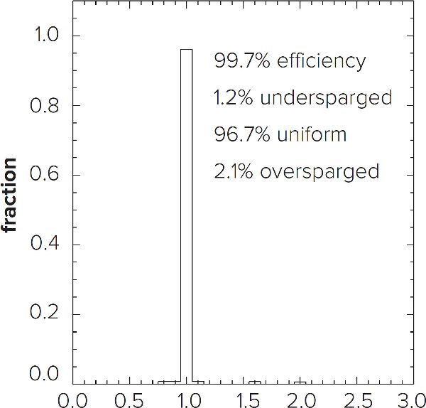
Figure F.7. Histogram showing the relative amounts of different percentages of unit flow as described by figure F.6. As expected, the histogram shows that the vast majority of the grainbed lies within the big white uniform region above the convergence zone.
Lauter Efficiency
Earlier we stated that 50% of the unit flow rate would only extract 50% of the sugar. However, we cannot say that a 200% flow rate will extract 200% of the sugar. If we assume that 100% of the unit flow rate extracts 100% of the sugar, then there is no more sugar to extract; higher flow rates do not extract anything further, except possibly tannins. If we add up all of the extraction rates from the different flow regions of the grain bed, we can determine the efficiency percentage for that configuration.
For example, if a single pipe manifold system lautered 5% of the grain bed at 40% of unit flow, 10% at 60%, 15% at 80%, and 70% of the grain bed at ≥100% of unit flow, the efficiency of that tun would be calculated as 90%:
(5 × 40) + (10 × 60) + (15 × 80) + (70 × 100) = 90% efficiency.
A “perfect” false bottom would lauter the entire grain bed with 100% of unit flow, because every region would have equal access to the drain, and would be 100% efficient. The computer model that applies the numerical model for fluid flow (see sidebar) estimates a real false bottom (⅛" holes on ¼" centers) to be 99.7% efficient (fig. F.7).
Lauter Uniformity
While efficiency gives a measure of the extract quantity, the uniformity gives a measure of its quality. To discuss uniformity, we look at three percentages of flow: flow less than 90%, flow between 90% and 110%, and flow greater than 110%. With these three percentages, we can compare different configurations that have similar efficiency, and determine if one configuration is more uniform than another. Regions of the grain bed with flow values between 90% and 110% are considered uniformly sparged, with values less than 90% being undersparged, and values over 110% oversparged. Generally, the percentage of oversparging is roughly the same as the percentage of undersparging for any one configuration.
Returning to our single pipe manifold example, let’s look at the histogram in figure F.5. From the histogram we can determine that only 56% of the grain bed is uniformly sparged, with 21% being undersparged, and 23% oversparged. This means 23% of the grain bed is subject to tannin extraction. But these percentages can be adjusted dramatically by tweaking a few variables.
Factors Affecting Flow
My thanks to Brian Kern—an astrophysicist at Caltech and a homebrewer—who co-developed this material with me.
The same computer model mentioned above was used to analyze 5,184 configurations of lauter tun and manifold in order to determine the primary factors for flow efficiency and uniformity. In descending order of influence, the factors are:
- • inter-pipe spacing,
- • wall spacing,
- • grain bed depth.
The analysis also determined that the pipe slots should always face down, being as close to the bottom as possible, because wort is not collected from below the manifold.
Inter-Pipe Spacing
By increasing the number of pipes across the width of the tun, you are effectively decreasing the inter-pipe spacing. Interestingly, analysis of the models (figures F.8–F.11) shows a nearly linear relationship between pipe spacing and both efficiency and uniformity, which peaks at a center-to-center pipe spacing of four times the pipe diameter. For a half-inch pipe, maximum efficiency and uniformity occur at a center-to-center spacing of two inches. Although optimum, it is not necessary for the pipes to be that close; the relationship between spacing and efficiency/uniformity starts to flatten out at three inches, or six times the pipe diameter. As can be seen in table F.1, only 1%–2% gains are realized by decreasing the pipe spacing from 3 to 2 in., although when the grain bed is shallow (<4 in.), the differences approach 5%.
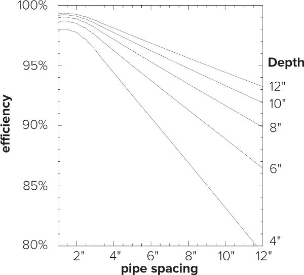
Figure F.8. Lautering efficiency as a function of pipe spacing and grain bed depth.
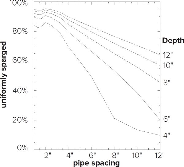
Figure F.9. Lauter flow uniformity as a function of pipe spacing and grain bed depth.
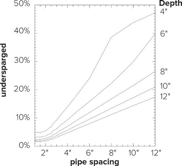
Figure F.10. Lauter flow under 90% as a function of pipe spacing and grain bed depth.
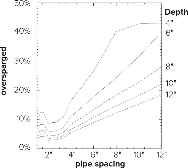
Figure F.11. Lauter flow over 110% as a function of pipe spacing and grain bed depth.
Table F.1—Effect of Inter-Pipe Spacing in 10"w × 8"h (25 × 20 cm) Grain Bed
| No. of pipes | Center-to-center spacing | Efficiency | Undersparged | Uniformly sparged | Oversparged |
|---|---|---|---|---|---|
|
1 |
10.00 |
91.7% |
21.5% |
55.7% |
22.8% |
|
2 |
5.00 |
96.2% |
9.6% |
79.7% |
10.7% |
|
3 |
3.33 |
97.8% |
5.5% |
89.0% |
5.5% |
|
4 |
2.50 |
98.6% |
3.4% |
92.1% |
4.5% |
|
5 |
2.00 |
98.9% |
2.7% |
93.0% |
4.3% |
Wall Spacing
The next most significant factor is the spacing of the pipes with respect to the walls of the tun. There are three ways to do this (fig. F.12):
- • Edge spacing—the two outermost pipes are placed flush against the walls and any other pipes are spaced evenly between them.
- • Even spacing—the spacing between the outer pipes and the walls is the same as the inter-pipe spacing.
- • Balanced spacing—the spacing between the outer pipes and the walls is half of the inter-pipe spacing.
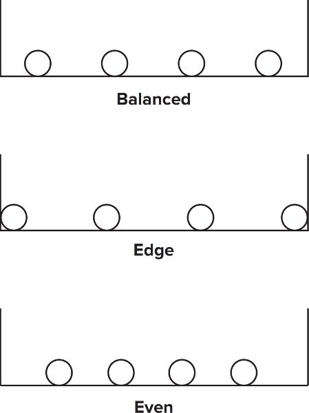
Figure F.12. Schematic showing three approaches to spacing of the pipes with respect to the walls of the lauter tun.
As you can see in table F.2, balanced spacing is the most efficient. Balanced spacing places the wall at half of the inter-pipe spacing so that flow velocity is symmetrical around every pipe in the manifold, and the manifold draws as uniformly as possible from the grain bed. Another way of looking at this variable is to say that, for a given tun width, balanced spacing covers the most area with the closest inter-pipe spacing using the least number of pipes. This is most significant for large inter-pipe spacings; at closer spacings the uniformity difference between balanced and edge spacing is smaller (5% or less). But with edge spacing, you need to be aware of the propensity for preferential flow down the walls to the drain. This phenomenon is often referred to as “channeling.”
Fluid mechanics describes a “boundary effect,” in which the flow resistance decreases at the wall, due to a lack of interlocking particles as a function of particle size (i.e., the wall is not grist, so there is more open area for flow at the wall). The boundary layer for crushed malt is about ⅛" (3 mm) wide. Likewise, if the edges of a false bottom do not conform to the tun walls, the flow will divert into the gaps. These low-resistance paths can result in a significant percentage of the sparge water bypassing the grain bed, which decreases the yield from each volume of wort collected. This means that balanced spacing is preferable to edge spacing for manifolds, and false bottoms should be fitted closely to the tun to minimize the effect.
Table F.2—Effect of Wall Spacing in a 10"w × 8"h (25 × 20 cm) Grain Bed
| No. of pipes | Wall spacing | Efficiency | Undersparged | Uniformly sparged | Oversparged |
|---|---|---|---|---|---|
|
2 |
Balanced |
96.2% |
9.6% |
79.7% |
10.7% |
|
2 |
Even |
94.5% |
14.1% |
66.6% |
19.3% |
|
2 |
Edge |
92.0% |
20.4% |
56.9% |
22.7% |
|
3 |
Balanced |
97.8% |
5.5% |
89.0% |
5.5% |
|
3 |
Edge |
96.4% |
9.0% |
80.3% |
10.7% |
|
3 |
Even |
96.2% |
9.7% |
76.3% |
14.0% |
|
4 |
Balanced |
98.6% |
3.4% |
92.1% |
4.5% |
|
4 |
Edge |
98.0% |
4.9% |
89.9% |
5.2% |
|
4 |
Even |
97.1% |
7.1% |
84.3% |
8.6% |
|
5 |
Balanced |
98.9% |
2.7% |
93.0% |
4.3% |
|
5 |
Edge |
98.6% |
3.4% |
92.0% |
4.6% |
|
5 |
Even |
97.7% |
5.3% |
87.6% |
7.1% |
Grain Bed Depth
The depth of the grain bed is the final significant factor affecting flow—not the total depth of the grain and sparge water, only the depth of the grain itself. For both false bottoms and manifolds, the amount of flow convergence depends only on the drain size and spacing. The size of the convergence zone does not change significantly with depth (pressure). The ratio of under-flow, uniform flow, and over-flow within the convergence zone are nearly constant, and the size (height) of the convergence zone is nearly constant. In the case of false bottoms, the drain features are quite small, so the convergence zone is narrow (less than a half inch in our model). But the drain features of manifolds are larger and more spread out, so the convergence zone is large and affects a larger proportion of the mash.
In other words, increasing the grain bed depth increases the proportion of the grain bed that is outside the convergence zone, which increases the proportion of uniform flow, which increases the extraction efficiency as a whole (table F.3). Thus, the efficiency of false bottoms (small convergence zones) are not significantly affected by grain bed depth, while manifolds (large convergence zones) are, although you can minimize the effect with a manifold by decreasing the inter-pipe spacing (by increasing the number of pipes) to reduce the height of the convergence zone.
Table F.3—Effect of Grain Bed Depth for a 10" (25 cm) Wide Grain Bed
| No. of pipes | Depth | Efficiency | Undersparged | Uniformly sparged | Oversparged |
|---|---|---|---|---|---|
|
1 |
4" (10 cm) |
83.2% |
43.8% |
13.4% |
42.8% |
|
1 |
6" (15 cm) |
88.9% |
29.9% |
38.4% |
31.7% |
|
1 |
8" (20 cm) |
91.7% |
21.5% |
55.7% |
22.8% |
|
1 |
10" (25 cm) |
93.3% |
17.2% |
64.5% |
18.3% |
|
1 |
12" (30 cm) |
94.4% |
14.3% |
70.4% |
15.3% |
|
1 |
24" (61 cm) |
97.2% |
7.2% |
85.1% |
7.7% |
|
1 |
48" (122 cm) |
98.6% |
3.6% |
92.5% |
3.8% |
|
5 |
4" (10 cm) |
97.8% |
5.4% |
86.1% |
8.5% |
|
5 |
6" (15 cm) |
98.5% |
3.6% |
90.7% |
5.7% |
|
5 |
8" (20 cm) |
98.9% |
2.7% |
93.0% |
4.3% |
|
5 |
10" (25 cm) |
99.1% |
2.2% |
94.4% |
3.4% |
|
5 |
12" (30 cm) |
99.2% |
1.8% |
95.3% |
2.9% |
|
5 |
24" (61 cm) |
99.6% |
0.9% |
97.7% |
1.4% |
|
5 |
48" (122 cm) |
99.8% |
0.5% |
98.8% |
0.7% |
For example: if you had only one pipe in a 10 in. wide tun with an 8 in. deep grain bed, the convergence zone is about 3.5 in. deep, and the percentage of uniform flow is 55.7%. If the grain bed is 48 in. deep, the convergence zone is still about 3.5 in., but the percentage of uniform flow is now 92.5%. With five pipes, the zone height is 0.5 in. and 90% of the flow is uniform at 8 in. depth. When you build a manifold lautering system, both the pipe spacing and wall spacing affect the actual size of the convergence zone, and the grain bed depth affects its relative size. To get the best performance from a manifold system you should optimize all three factors.
The four plots in figures F.8 and F.11 summarize the analysis of all the numerical models for inter-pipe spacing, wall spacing, and grain bed depth, for ½" diameter pipes. Each plot shows the behavior of the stated quantity as a function of center-to-center pipe spacing and as a function of grain bed depth. The relationships are nearly linear except at close pipe spacings and shallow grain bed depths.
Designing Pipe Manifolds for Continuous Sparging
To summarize:
- • The manifold should cover most of the floor of the lauter tun.
- • The manifold should have a pipe spacing of 2–3 in. (5–7 cm).
- • Use balanced spacing to get the best results with the fewest pipes.
- • Choose a cooler size that will give a good grain bed depth for your typical batch. I recommend a depth of 4–12 in. (10–30 cm).
In a circular cooler, the best shape for a manifold is a circle divided into quadrants, although an inscribed square seems to work just as well (see fig. E.7). In a rectangular cooler, the best shape is rectangular with several legs to adequately cover the floor area (fig. F.13). Whether circular or rectangular, when designing your manifold, keep in mind the need to provide full coverage of the grain bed while minimizing the total distance the wort has to travel to reach the drain.
In addition, it is very important to avoid channeling of the water down the sides from placing the manifold too close to the walls. The distance of the outer manifold tubes to the cooler wall should be half (or slightly greater) of the manifold tube spacing. This results in water along the wall not finding a shorter path to the drain than wort that is dead center between the tubes.
The transverse tubes in the rectangular tun should not be slotted. The longitudinal slotted tubes adequately cover the floor area and the transverse tubes are close enough to the wall to encourage channeling. The slots should face down—any wort physically below the slots will not be collected. In a circular tun, the same guidelines apply, but if you are using an inscribed square the transverse tubes can be slotted where they are away from the wall.
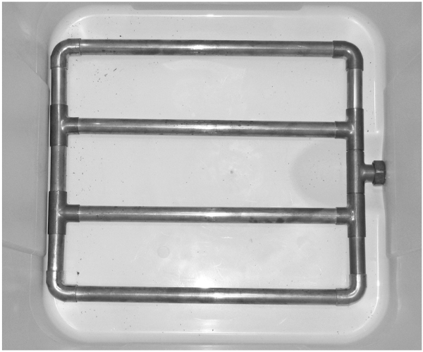
Figure F.13. Multi-pipe manifold in square cooler.
Designing Ring Manifolds for Continuous Sparging
Ring-shaped manifolds or stainless steel braids are an elegant looking system for cylindrical beverage coolers, but how efficient are they? It turns out that they are pretty good if the balanced spacing concept is applied. For a single ring, balanced spacing means having an equal volume inside and outside the ring. The calculate the diameter of a ring that will divide the tun volume in half, simply multiply the tun diameter by 0.707:
Ring diameter = 0.707 × tun diameter
The chart in figure F.15 plots the efficiency quantities of rings and false bottoms in a Sankey keg as a function of diameter. The total diameter of a Sankey keg is 15 in. (38 cm), so the half volume diameter is 10.6 in. (27 cm). It is interesting to note that a single ring is more efficient than a false bottom until the false bottom diameter is at least 80% of the tun diameter. These ratios hold true for any tun diameter. If more rings were added in a balanced spacing manner, the efficiency would improve and approach that of false bottoms, just like rectangular manifolds in rectangular coolers.

Figure F.14. Braided ring in cylindrical cooler.
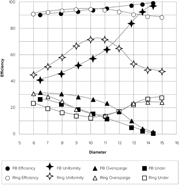
Figure F.15. Plotting the efficiency quantities of rings and false bottoms (FB) in a 15 in. diameter Sankey keg as a function of ring or FB diameter.