CHAPTER 8
Loans and the Theory of Credit

Much of the credit research presented thus far has been empirical, using historical data to drive an understanding of credit return and risk. However, credit can also be understood from a theoretical perspective, using option‐pricing theory to explain and measure credit return and risk. This chapter reviews some basic theoretical underpinnings of credit and ties its conclusions to market behavior.

The chapter begins with a review of the Merton model for pricing corporate debt; shows how it can be applied to calculate credit risk premiums for middle market corporate loans, including sensitivity analysis; estimates credit risk using Monte Carlo simulation; and finally, tests risk findings against historical risk measures.

This research approach can be helpful in several ways. For example, understanding the Merton model better informs investors of loan pricing and its determinants. Take the tightening of yield spreads for credit securities relative to comparable maturity Treasury securities (also called spread compression), for example, which is generally attributable to capital inflows but instead could be explained by a rise in the risk‐free rate. Another application is determining return and risk expectations for less familiar debt instruments such as second‐lien and mezzanine loan structures, which can be estimated through simulation techniques where empirical data is not available.

To better understand the implications of the current covenant‐lite trend, an extension of the Merton model called the Black–Cox model is reviewed. The Black–Cox model provides a method for pricing covenants and, in so doing, offers a method for pricing (in yield equivalent) the cost of covenant‐lite loans. For example, the application of the Black–Cox model shows that a trend toward covenant light structures reduces return by approximately 1% but that cost varies considerably and directly with the loan level leverage.

Like capital asset pricing model (CAPM) and Black–Scholes, the Merton and Black–Cox models have withstood the test of time but remain imperfect approximations of a complex credit world. Nonetheless, this chapter shows that theoretical guideposts exist to better understand and measure credit‐driven investment opportunities and risks.

THE MERTON MODEL

Current corporate credit theory remains almost entirely based upon Robert Merton's 1974 adaptation of the Black–Scholes option pricing formula to corporate credit.¹ Merton showed that the same formula for pricing stock options could be used for pricing bonds by associating the level of corporate debt with the exercise price of a stock option.

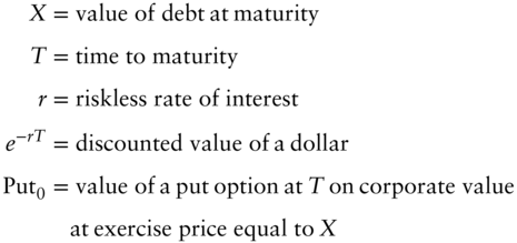
In Merton's world, the corporate lender can be thought of as (i) providing the corporate borrower a fixed amount of debt capital, expecting full repayment at maturity plus interest, plus (ii) selling the corporate borrower a put option and receiving a premium, giving the borrower the right to repurchase the debt at maturity for the then value of corporate assets. At maturity, the borrower's put option only has value if the value of corporate assets is less than the value of the corporate debt, and the debt can be settled in full by remaining corporate assets.

In Merton's world, the expected risk of default is fully absorbed by the corporate borrower through the premium cost of the put. Hence, the principal value of the debt becomes technically default‐free and the interest rate in (i) above is deserving only of the risk‐free rate of return to compensate for the time value of money. Hence, the value of corporate debt can be written as:

(8.1)

The annuitized value of  in Equation 8.1 can be viewed as the annualized credit risk premium. However, Merton provides a more direct calculation of the credit risk premium in Equation 8.2:

(8.2)

As expected, Equation 8.2 has the same look as Black–Scholes, but here the contents in the brackets represent a weighted average of the current asset coverage ratio and an asset coverage ratio equal to 1.0, the default point. The weights () depend upon time to maturity, firm risk, and debt levels. More weight is given to the debt coverage ratio as debt increases. The first term amortizes the credit premium over the life of the loan.

Exhibit 8.1 applies Merton's formula to a hypothetical middle market corporate loan. We assume a five‐year loan, a borrower whose assets (unlevered firm) exhibit a 40% standard deviation, and a 1.75% riskless rate of interest over the life of the loan. Because we also are modeling a private loan, we assume a 2.00% liquidity premium and a 0.5% annualized original issue discount (OID), values that are consistent with research on middle market loans presented in Chapter 9.

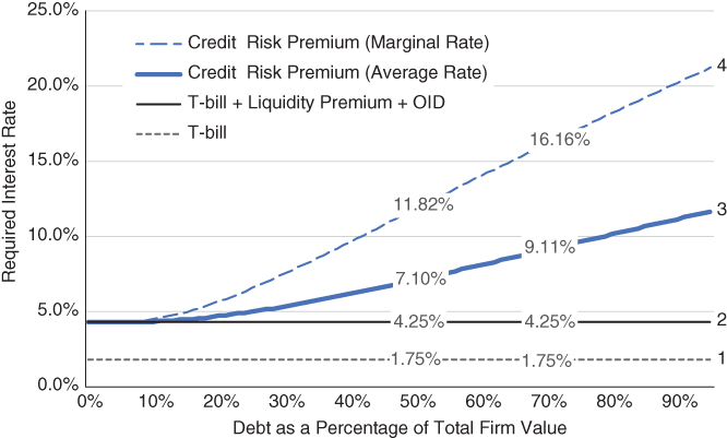
EXHIBIT 8.1 Merton model of debt costs and loan‐to‐value ratios for private debt.

Line 3 in Exhibit 8.1 is the investor's required interest rate at varying leverage levels to compensate for time, liquidity, and credit risk. For example, in an efficient market a lender would require a 7.10% yield for a private loan equal to 50% of total firm value. That 7.10% would be comprised of a riskless 1.75% for the time value of money, 2.00% for the loss of liquidity, 0.50% for the cost of creating the loan, and 2.85% to compensate for default risk. As expected, yield increases as debt increases. At 70% debt, a level reflective of some unitranche loans, the yield increases to 9.11%.

The representation of yield in line 3 is an average yield because it represents the composite pricing of debt capital from the first dollar (1% of total assets) through the last dollar (i.e., the 1% of debt capital that brings total debt from 49% to 50%). Theoretically, each incremental dollar of debt brings greater risk and should have a greater yield. Marginal yield represents the pricing of incremental debt capital and is shown in line 4. For example, the yield required for the last 1% of debt capital before a cumulative 50% of total assets is reached equals 11.82%. For a unitranche loan seeking 70% debt capital, the last marginal 1% requires a yield equal to 16.16%.

Marginal yields are useful for several reasons. First, they inform investors that the high yields they see reported for second‐lien, subordinated, and mezzanine debt are necessary to compensate for credit risk. Second, they help investors understand the yield differences for varying senior debt structures – i.e., super‐senior, senior, stretch senior, and unitranche – each having differing attachment points. For example, a 70% unitranche loan that sells a 20% “first out” loan participation raises the yield on its “last out” by almost two percentage points, from 9.11% to 10.88%. Third, marginal yields inform investors as to the importance and pricing of covenants that offer lenders protection against potential adverse marginal use of corporate assets by borrowers.

It is also instructive to understand how credit risk premiums change with the three underlying inputs: firm volatility, the risk‐free rate, and time.

VOLATILITY

Exhibit 8.2 plots just the credit risk premium component of return at firm risk levels of 30%, 40%, and 50%. Firm volatility levels of 30% and 50% represent approximately one standard deviation from the mean.²

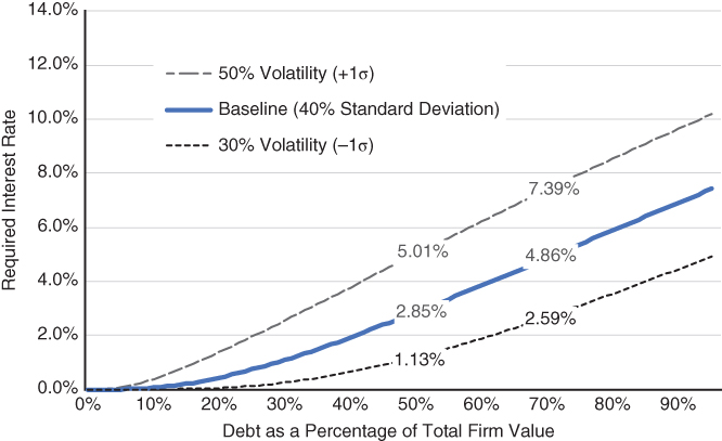
EXHIBIT 8.2 Credit risk premium and firm risk.

Credit risk premiums are quite sensitive to perceived market volatility. At a 50% debt to firm value level, credit risk premiums can double or halve with major moves in the VIX.

Firm risk is generated primarily from three sources: overall market conditions, firm specific conditions, and industry conditions. Overall market conditions would likely set and move risk premiums similarly across all loans. Firm specific conditions, by definition, are unique to individual companies and would move risk premiums singularly. Industry conditions impact the loan pricing of borrowers as a subgroup within the same industry.

Exhibit 8.3 shows firm volatility estimates across industry groups based upon companies in the Russell 2000 Index covering the 11‐year period from 2007 through 2017. Individual firm volatility (standard deviation) is calculated by adjusting firm stock volatility over the measurement period for firm leverage (debt to total assets) over the measurement period. The average volatility for all firms within the same industry is calculated and reported in Exhibit 8.3, ordered from highest volatility industry to lowest volatility industry. Average volatility for all Russell 2000 companies is reported as well.

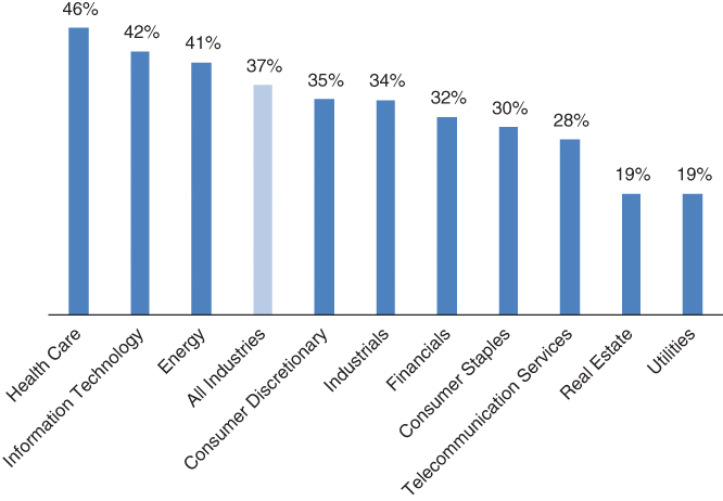
EXHIBIT 8.3 Firm volatility (standard deviation) by industry group.

The disparity in firm volatility by industry coupled with the sensitivity of credit risk premiums to firm volatility suggest that industries should each carry substantially different yields, everything else being equal. For example, the same 50% debt ratio loan should carry a 4.11% risk premium for the average healthcare borrower but only 0.16% for the average utility company. Not surprisingly, lenders that specialize tend to select the higher volatility industries where the reward from skilled underwriting is potentially much greater.

RISK‐FREE RATE

Exhibit 8.4 shows how the credit risk premium changes with the risk‐free rate. Exhibit 8.4 focuses only on the credit risk premium itself and does not include how the risk‐free rate directly impacts the base rate on floating rate loans.

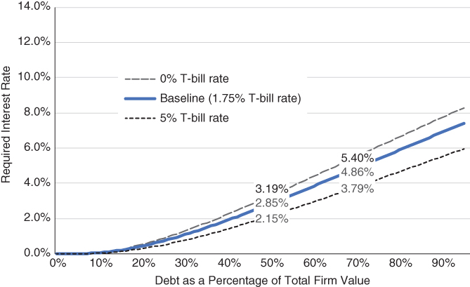
EXHIBIT 8.4 Credit risk premium and the risk‐free rate.

Credit risk premiums are inversely correlated to the risk‐free rate. At a 50% debt to firm value level, the credit risk premium is 3.19% at a 0% T‐bill rate and 2.15% at a 5% T‐bill rate. A higher risk‐free rate lowers the effective strike price of the put sold to borrowers by lenders. The lower strike price makes the put less valuable, lowering the option premium and, therefore, the credit risk premium received by the lender.

As Exhibit 8.4 shows, the impact of rising interest rates on credit spreads is not inconsequential. At the 50% debt level, an increase in the risk‐free rate from 0% to 5% lowers the credit risk premium by 1.04%. At a 70% debt level, the credit risk premium falls by 1.61%. A 20% loan subordinated to a 50% senior loan would see its credit risk premium fall by 3.03%, from 10.92% to 7.89%, from a 0% to 5% T‐bill rate change.

The relationship described in Exhibit 8.4 may explain some of the yield spread compression that has been coincident with rising short rates.

TIME TO MATURITY

Exhibit 8.5 describes the relationship between credit spreads and time to maturity. Unlike volatility and the risk‐free rate, which change credit spreads in the same direction, across debt to total firm assets, time to maturity changes direction.

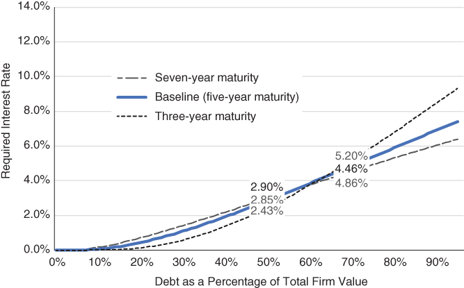
EXHIBIT 8.5 Credit risk premium and time to maturity.

Exhibit 8.5 mostly confirms conventional thought that longer maturity loans are riskier for the lender and require higher spreads. However, at very high debt ratios (60% and above in our example), longer maturity loans are less risky.

ESTIMATING LOAN RISK

The Merton model is also useful for estimating the risk characteristics of a corporate loan. To demonstrate this, stock returns are simulated, and the Merton formula is applied to show the impact on corporate loan pricing.

Simulation inputs are:

1. Middle market corporate loans with a five‐year maturity.
2. Floating interest rates so the five‐year, risk‐free bond has zero risk (no duration).
3. Annualized firm‐level risk equal to 37%, derived in the following way. We calculate the stock risk of every company in the Russell 2000 small stock index over the past 10 years ending December 31, 2017, finding a 47% average. Since the Merton model requires firm‐level volatility, not stock volatility, we convert the 47% stock risk to an estimate of firm level risk by deleveraging using the average 0.23x Russell 2000 debt‐to‐total assets ratio over the same 10‐year period. Deleveraging produces a 37% annualized risk estimate for the average Russell 2000 company. Russell 2000 companies were selected as a proxy for US middle market companies because their median earnings before interest, taxes, depreciation, and amortization (EBITDA) of $57 million is at roughly the midpoint of the $10 million to $100 million EBITDA range that generally defines the corporate middle market. The difference is that Russell 2000 companies are exchange traded while most middle market borrowers are private companies.
4. The 37% firm‐level risk estimate is divided into two risk sources: market‐related risk (beta) and nonmarket idiosyncratic risk. Market risk is assumed to be 19%, equal to the risk of the Russell 2000 Index over the same 10‐year period. Knowing that, by definition, market and non‐market risks are independent of each other, the calculation for the non‐market risk for the average middle market company equals 32%.³

Exhibit 8.6 provides simulation results for three loans. The first represents a senior, first‐lien loan with a principal value equal to 50% of initial firm assets. The second represents a unitranche loan, intended to incorporate first‐ and second‐lien loans into one, with a principal value equal to 70% of firm assets. The third loan is second lien with a value equal to 20% of initial firm assets and with lien protection above the 50% asset value. Results are based upon 1,000 trials.

EXHIBIT 8.6 Simulation results for a hypothetical first‐lien, unitranche, and second‐lien loan.

	First Lien	Unitranche	Second Lien
Loan size	50% of firm assets	70% of firm assets	20% of firm assets
Recourse	All firm assets	All firm assets	Firm assets above 50% first lien
Risk (std. dev.)	8.54%	12.04%	24.88%
Corr. w/ Russell 2000	0.45	0.47	0.48
R‐Square	20%	21%	22%
Beta	0.19	0.27	0.57
Convexity	−0.26	−0.30	−0.42
Skew	−1.01	−0.64	−0.23

Exhibit 8.7 displays the simulation outcomes for the first lien and second lien graphically.

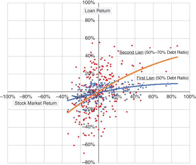
EXHIBIT 8.7 Simulation results for hypothetical first‐lien and second‐lien loans.

Exhibits 8.6 and 8.7 together provide useful guidance on what to expect in terms of risk from different loan structures. Not surprisingly, risk (standard deviation) increases from 8.54% for a senior loan to 12.04% for a unitranche loan and 24.88% for a second‐lien loan. However, correlation and R‐square with the Russell 2000 Index remain largely unchanged across the three loan types as equity risk represents a roughly constant percentage of total risk. Finally, equity beta increases from 0.19 for a senior loan to 0.27 for a unitranche loan and 0.57 for a second‐lien loan. Loans do act more like equity further down in the capital structure.

Loans also possess other less desirable risk features. The simulated loan returns feature negative convexity, consistent with the short volatility nature of the short‐put feature in Equation 8.1. However, the negative convexity is not severe, and is far less than what is found in hedge fund returns.⁴ Loans also display a negative skew, or downside tail in the distribution of returns. But unlike risk and convexity, skew improves as credit quality declines.

ESTIMATING LOAN PORTFOLIO RISK

Exhibits 8.8 and 8.9 contain risk characteristics for a portfolio of loans, which is likely of greater interest. We simulate returns for portfolios of senior loans, unitranche loans, and second‐lien loans, assuming 100 loans in each portfolio. As before, we simulate equity market risk and company specific risk separately.

EXHIBIT 8.8 Simulation results for hypothetical first‐lien, unitranche, and second‐lien 100‐loan portfolios.

	First Lien	Unitranche	Second Lien
Loan size	50% of firm assets	70% of firm assets	20% of firm assets
Recourse	All firm assets	All firm assets	Firm assets above 50% first lien
Risk (std. dev.)	5.67%	8.29%	17.78%
Corr. w/ Russell 2000	0.73	0.74	0.75
R‐Square	54%	55%	57%
Beta	0.22	0.32	0.70
Convexity	−0.39	−0.48	−0.80
Skew	−0.81	−0.55	−0.26

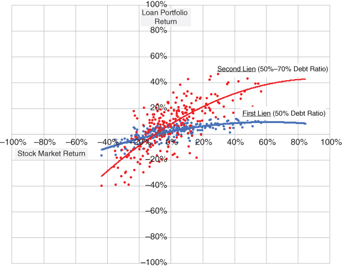
EXHIBIT 8.9 Simulation results for hypothetical first‐lien and second‐lien loan portfolios.

Equity market risk impacts all loans the same, at least directionally. Conceptually, company specific risk should be independent with zero correlation across companies. However, we assume the same 0.25 cross correlation for all 100 loans instead of a zero correlation because, in our experience, there exist common factors beside the market factor that tend to push returns in the same direction. These common factors could include industry, liquidity, and size factors. Our choice of 0.25 is consistent with values found for hedge fund returns after market returns are stripped from total returns. With these assumptions, the nonmarket firm level risk for a portfolio of loans equals 16% compared to 32% for a single corporate borrower. The simulation results in Exhibits 8.8 and 8.9 are based upon 1000 trials.

Portfolio diversification reduces nonmarket risk, causing higher beta, correlation, and R‐square values for loan portfolios in contrast to individual loans. Convexity worsens but skew improves slightly.

TESTING THE MERTON MODEL

The simulated loan portfolio risk estimates contained in Exhibit 8.9 are next compared to risk calculations for actual returns reported for two corporate credit indexes: the S&P/LSTA Leveraged Loan Index and the Bloomberg Barclays High Yield Bond Index. The first index is comprised of traded floating‐rate bank loans, generally senior in credit standing, while the second index is comprised of traded fixed‐rate corporate bonds, generally subordinated to bank loans. Our risk calculations are based on monthly returns from January 2000 through December 2017.

In addition, because the Bloomberg Barclays High Yield Bond Index returns are fixed rate, their monthly returns are impacted by changes in longer maturity interest rates. By contrast, our simulated returns assume floating rates. To convert the fixed‐rate Bloomberg Barclays High Yield Bond Index to floating rate, the duration‐equivalent monthly Treasury bond return is subtracted from the monthly Index return. The result should be what the Bloomberg Barclays High Yield Bond Index would have returned if the underlying bonds were floating rate rather than fixed rate.⁵

Exhibit 8.10 compares the simulated loan portfolio risk characteristics with calculations based on actual index returns.

EXHIBIT 8.10 Simulated versus actual risk calculations.

	(Exhibit 8.7) Simulated First Lien	(Exhibit 8.7) Simulated Second Lien	S&P LSTA Leveraged Loan Index	Duration‐Adjusted Bloomberg Barclays High Yield Bond Index
Risk (std. dev.)	5.67%	17.78%	6.21%	11.01%
Corr. w/ Russell 2000	0.73	0.75	0.47	0.68
R‐Square	54%	57%	22%	47%
Beta	0.22	0.70	0.15	0.39
Convexity	−0.39	−0.80	−1.35	−2.26
Skew	−0.81	−0.26	−2.03	−1.01

A comparison of the simulated first‐lien risk calculations and the S&P LSTA Leveraged Loan Index reveals both similarities and differences. Risk values (standard deviations) are very similar as are the betas. Convexity and skew are higher for the S&P LSTA Leveraged Loan Index but that is likely because the Russell 2000 Index itself displayed some of those same characteristics during the measurement period, which probably magnified the S&P LSTA Leveraged Loan Index values.

A comparison of the simulated second‐lien risk calculations and the duration‐adjusted Bloomberg Barclays High Yield Bond Index also includes similarities and differences. Importantly, higher risks and higher betas for subordinated debt are exhibited in both simulated and duration‐adjusted actual returns. The biggest difference is the much higher 17.78% risk level for simulated second lien versus 11.01% for the duration‐adjusted Bloomberg Barclays High Yield Bond Index. This difference is likely due to an inexact match in debt ratios between our hypothetical second‐lien loan and the actual debt ratio specifications for the Index.

MERTON MODEL WITH COVENANTS

Easy credit conditions not only result in spread narrowing, but also relaxation in loan covenants. An extension of the Merton model by Fischer Black and John Cox⁶ (Black–Cox) addresses the value of covenants where the Merton model was covenant‐free. The Black–Cox model is an important tool for lenders who want to understand the cost of foregoing customary covenants late in a credit cycle.

The Merton model has no provision for bankruptcy prior to loan maturity. Loan covenants vary in type but all act to trigger a default or restructuring prior to maturity. By doing so, covenants can protect possible further erosion in firm assets and enhance recoveries. They can also accelerate cash flow to the lender, thereby creating value.

Black–Cox extends the Merton model to include covenants, also using option‐pricing theory.⁷ Covenants are intended to protect the value of firm assets and ultimately can terminate the loan through default before maturity if firm assets fall below loan face value. Ideally, the loan face value becomes a barrier for firm assets after which default is declared in a covenant tight world. More likely, the look‐back nature of covenants results in a barrier that falls below face value, but once the covenant barrier is broken the lender “takes the keys” and replaces the equity holder.⁸ Black–Cox argue that this dynamic mirrors a “down‐and‐in” call option given to the lender and can be valued in the same way.

Exhibit 8.11 provides an example of a down‐and‐in option.

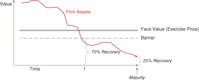
EXHIBIT 8.11 Illustration of down‐and‐in option.

At loan underwriting (time = 0) firm assets are well above face value, but take a declining path to equal just 25% of loan value at maturity. Under the Merton model, default would occur at maturity and the lender would recover just 25% of principal.

In the Black–Cox model, loan covenants produce a value barrier, giving lenders the opportunity to force borrowers into default before maturity. In our example, covenants allow the lender to force default at time t where recovery equals 70% of principal, saving 45% of value (70% minus 25%). Our example is one of many scenarios that could play out, including some where asset recovery makes early default costly.

Conceptually, covenants give the lender the right to buy the firm at an exercise price equal to the face value of the loan once covenant terms have been violated, which is represented by firm assets falling below the barrier value. The representation of loan principal as exercise price means that through default the lender pays for the firm assets by absolving the borrower of principal repayment. This description fits the standard options pricing model except that the option comes into existence and has value only on the condition that firm assets drop through a barrier created by the loan covenants. The Black–Cox model values the “down and in” option and in so doing, the value of the covenant.

In Exhibit 8.12 we take the example in Exhibit 8.1 but add a covenant package that creates a barrier equal to 60% of the face value of the loan. We select 60% because it approximates the historical average recovery rate on broadly syndicated leveraged loans, which generally come with covenants.

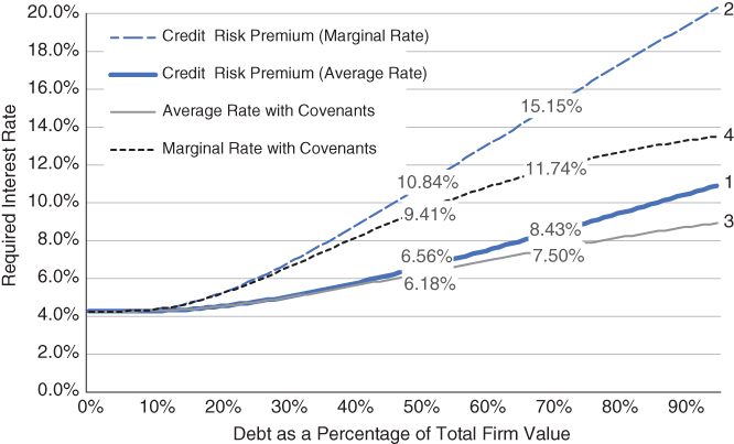
EXHIBIT 8.12 Debt costs with/without covenants (a theoretical representation using the Black–Cox model).

Lines 1 and 2 are repeated from Exhibit 8.1 and show average and marginal loan rates using the Merton model without covenants. Lines 3 and 4 are added and represent the average and marginal loan rates using the Black–Cox model with covenants. As expected, lender protections from covenants add value to a loan as measured by a down‐and‐in call option and convert to a lower interest rate required by the lender. For example, a senior loan representing 50% of firm assets would require a 6.56% rate without covenants and a 6.18% rate with covenants. Covenants could be said to be worth an extra 0.38% (6.56% minus 6.18%).

Observe that covenants become much more important to the lender as a loan stretches to higher ratios of firm value. At a 70% loan to asset value, the loss of covenant protection requires an additional 0.93% of yield (8.43% minus 7.50%), compared to 0.38% for the 50% loan.

Finally, marginal rates without and with covenants are represented by lines 2 and 4, respectively, and point to their critical importance in pricing second‐lien loans. For example, a second‐lien loan representing 20% of firm assets with a 50% attachment point would require a yield equal to 13.11% without covenants and 10.80% with covenants, a 2.31% difference.

Understanding the imprint of covenants on loan pricing would seem critical in an environment trending toward covenant lite, because it represents an erosion in expected return not reflected in headline credit spreads.

Covenants also reduce many risk measures for a portfolio of loans. Exhibit 8.13 compares risk statistics for a diversified portfolio of unitranche loans without covenants (see Exhibit 8.8) and with covenants.

EXHIBIT 8.13 Simulation results for hypothetical unitranche 100‐loan portfolio with and without covenants.

	Unitranche without Covenants	Unitranche with Covenants
Loan size	70% of firm assets	70% of firm assets
Recourse	All firm assets	All firm assets
Risk (std. dev.)	8.29%	6.20%
Corr. w/ Russell 2000	0.74	0.73
R‐Square	55%	53%
Beta	0.32	0.24
Convexity	−0.48	−0.11
Skew	−0.55	−0.39

Covenants lower risk and beta and improve convexity and skew. What doesn't really change is the correlation and R‐Square with stocks. In summary, covenants play an important role in both the pricing (yield) and risk of loan portfolios and can be valued by the Black–Cox model.

The Merton model provides a useful framework for understanding the pricing of corporate loan yield spreads. Coupled with simulation methods, investors can develop useful estimates of return and risk for loans of differing credit seniority, including covariances useful for multi‐asset optimization.

The Merton model reveals that credit risk premiums (yields) rise rapidly as loan leverage ratios increase and that expectations of underlying firm risk, whether market, industry, or firm‐specific, can produce significant differences in risk premiums. Simulation confirms that corporate loans of varying leverage levels all have high correlations with the stock market. However, senior loans display much lower levels of risk compared to subordinated loans.

The Black–Cox model shows how to value loan covenants and measure the impact of covenant‐lite structures. A reasonable estimate for the value of covenants is approximately 1% per annum, but that value will increase (decrease) with loan seniority and leverage ratios.

NOTES

1 Robert C. Merton, “On the Pricing of Corporate Debt: The Risk Structure of Interest Rates,” The Journal of Finance (May 1974).

2 The standard deviation of the VIX Index, a measure of equity market risk, equals 8.11% when measured monthly over the 20 years ending 2017. We estimate that the average beta for middle market companies equals 1.2, so that one standard deviation of market risk applied to middle market companies equals 9.73%. We assume company‐specific risk does not change and add (subtract) 10% to the 40% average firm risk.

3 0.32² = 0.37² + 0.19², assuming zero correlation between market and nonmarket risk.

4 For example, Cliffwater calculates an average convexity value equal to −0.78 for a diversified group of 600 larger hedge funds covering a five‐year period ending December 31, 2017.

5 A monthly Treasury bond return of equal duration to the Bloomberg Barclays High Yield Bond Index is calculated using durations and returns for the five‐year maturity Treasury and three‐month T‐bill.

6 Fischer Black and John C. Cox, “Valuing Corporate Securities: Some Effects of Bond Indenture Provisions,” The Journal of Finance (May 1976).

7 Fischer Black is the same author of the Black–Cox and Black–Scholes models.

8 At barrier breaches, lenders more often extract value from borrowers other than “taking the keys,” including special payments or yield adjustments, whose potential value can also be represented by Black‐Cox.