CHAPTER 14
Loan Valuation
How accurate are valuations in the absence of a tradable market for middle market loans? This is an important question for most investors in direct corporate loans for several reasons. First, many investors in public business development companies (BDCs) focus on the price‐to‐NAV ratio (the BDC market price divided by net asset value) as a potential measure of under‐ or overvaluation, signaling a buy or sell opportunity. If net asset value is incorrect, so is the valuation signal. Second, manager fees are based upon net asset value so mistakes in valuation can potentially cause fee overpayments. Third, some direct lending pooled vehicles allow investors to purchase or sell units at net asset value. Private BDCs and other registered and nonregistered, open‐end pooled vehicles are examples. For example, if net asset value is overstated, the excess value is passed from the new shareholders making investments to existing shareholders, and at the same time excess value is passed from existing shareholders to withdrawing shareholders. Excess value flows in the opposite direction when net asset value is understated. This chapter addresses how direct loan values are determined and whether investors can rely on them.
As background, the Financial Accounting Standards Board (FASB) defines asset value as fair value,1 prescribed by ASC 820 most recently in 2011. ASC 820 defines fair value as “the price that would be received to sell an asset or paid to transfer a liability in an orderly transaction between market participants at the measurement date.” In outlining a discovery process that will find fair value, ASC 820 segregated assets into three categories (level 1, level 2, and level 3), each with a different process for determining fair value.
Level 1 assets are liquid assets with valuations based on quoted prices readily available in active markets. Level 1 assets typically include listed equities, listed derivatives, mutual funds, and any other assets that have a regular mark‐to‐market pricing mechanism, generally via a central exchange. Investors should have high confidence in level 1 valuations, except perhaps during extreme events. Level 2 assets generally trade in inactive markets and rely upon values (quotes) provided by market participants rather than real time transactions on a central exchange. These assets are often priced through indicative quotations from multiple broker–dealers and then averaged. Examples of level 2 assets include credit default swaps and corporate debt. Most derivative securities are considered level 2 assets even though the valuation for the underlying security may be readily available on a central exchange. Level 3 assets are generally those that are not traded or traded infrequently and therefore fair value cannot be determined by market‐related activity or inputs. The fair value of level 3 assets can only be estimated by using significant assumptions as inputs to a valuation model.
Direct middle market corporate loans are level 3 assets. There may be some exceptions when the direct loans are lightly traded, in which case they might be treated as level 2. While ASC 820 gives broad discretion in setting fair value for level 3 assets, there are several straightforward models available to price loans. The key inputs are the most recent borrower financials, recent changes, and most likely a valuation model that maps the circumstances of the loan being valued to a pool of other loans with similar circumstances that have a credit rating. Pricing can then be discovered once a rating equivalent is agreed upon. Importantly, asset managers develop written valuation policies that guide how it is valuing level 3 assets and a compliance function confirms that these policies are being consistently followed.
Common practice is for direct loans to be valued quarterly. Another, not dissimilar valuation process is used for determining the value of liabilities if financing is used. Net asset value equals the fair value of assets minus the fair value of liabilities. It is also common for the asset manager to use an independent external valuation firm to value its level 3 loans at least once a year with the loan manager setting values during the off quarters. Best practice is quarterly independent valuations, though these can be costly and so managers generally weigh the net benefits of this practice to shareholders.
The quality of ASC 820 fair value protocols as they apply to level 3 assets and direct US middle market corporate loans in particular, can be tested by comparing, in the aggregate, quarterly pricing for high‐yield bonds and broadly syndicated bank loans, both of which are level 2 assets, with the fair value determination of direct loans captured by the Cliffwater Direct Lending Index (CDLI). More granular comparisons of individual loans or groups of loans with equivalent level 2 loans might reach different conclusions, but the comparison in Exhibit 14.1 between direct loan values and traded high‐yield bonds and bank loans should provide guidance about the pricing behavior and accuracy of diversified loan portfolios over time.
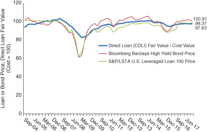
EXHIBIT 14.1 Price comparison for direct loans, high‐yield bonds, and bank loans, March 2004 to December 2017.
Quarter valuations for the three indices are plotted in Exhibit 14.1. Casual inspection suggests that pricing for direct loans, as measured by the CDLI, tracks the short‐term directions of high‐yield bonds and bank loans, and for the most part direct loan values lie between their level 2 counterparts. The exceptions are the 2008 global financial crisis (GFC) and, to a lesser extent, the 2015–2016 oil crisis. The valuation divergence for direct loans during the oil crisis was likely due to the difference in energy sector weights between the CDLI, where energy represented less than 5% of the index, and high‐yield bonds and bank loans, where energy represented well over 10% of those indexes.
The markedly higher valuations for direct loans during the GFC require a different explanation. At December 31, 2018 there was a 25‐point difference in valuation, which surely did not originate from changing fundamentals of the underlying companies across the three Indices. At the time, liquid high‐yield bonds and loans were popular collateral in structured vehicles carrying high leverage. The unwinding of these vehicles caused selling pressure and lower prices on level 2 risky assets that did not impact direct loans, which were held in banks, insurance companies, and closed‐end BDCs. Effectively, direct loan values were set to reflect ASC 820 orderly transaction pricing rather than the market dislocation pricing occurring at the time. It is interesting that after the GFC the FASB added to its level 3 pricing guidance the concept of risk adjustment in pricing when there is significant measurement uncertainty. This may change valuation behavior for direct loans during the next market downturn.
The direct loan valuations in Exhibit 14.1 also appear less volatile, apart from the 2008 GFC. This lower volatility is also reflected in the calculation of return volatility reported in Exhibit 3.1, where direct loans had a 3.5% standard deviation compared to 10.2% for the S&P/LSTA Leveraged Loan Index and 10.7% for the Bloomberg Barclays High Yield Bond Index. Direct middle market loans may in fact be less volatile than these publicly traded bank loans and bonds. But an alternative explanation could be that the level 3 valuation process might somehow be flawed and that those setting fair value are not doing so conditioned only on information as of the valuation date, but also implicitly take account of past prices and future expectations. If true, this creates a smoothing of prices over time, lowering the measured standard deviation of return.
A test for the presence of smoothing would be a positive finding of serial correlation in direct lending returns. Serial correlation measures the correlation of current returns with returns from prior periods. If there is no smoothing, serial correlation equals zero. This is the ideal random‐walk world, where past prices do not influence current or future prices. If serial correlation is positive and equal to 0.50, for example, it means that past prices do explain current pricing to a degree equal to 25% (equal to 0.502).
Returns can also be found to have correlation not only with the immediate prior quarterly return, but quarterly returns extending back in time. A common manifestation of this effect used to occur in private real estate and private equity returns where serial correlation persisted up to a four‐quarter lag. This produced significant smoothing in returns, causing risk calculations based upon these returns to be understated. The cause of the serial correlation in these smoothed returns was intermittent independent valuations, most done annually, without the rigorous guidelines of ASC 820. Over the last decade the integrity of valuations has become a greater priority for all private asset classes.
The integrity of direct loan valuations can be tested by measuring serial correlations of various time lags for direct lending quarterly returns. Quarterly CDLI price returns, not total returns, are used because valuation impacts change in price but not income. The CDLI quarterly price return equals realized plus unrealized capital gains (losses) divided by net asset value.
Serial correlations in CDLI price returns equal to 0.38, 0.09, 0.14, and 0.05 are found for one‐quarter lag, two‐quarter lag, three‐quarter lag, and four‐quarter lag, respectively. In a regression where the CDLI quarterly price return is the dependent variable and each of the four prior quarter price returns are independent variables, only the immediate prior quarter shows any level of statistical significance with a t‐statistic equal to 2.23. Keeping only the immediate prior quarter price return as the only independent variable increases the t‐statistic to 2.91.
These measurements suggest modest and short‐lived smoothing in direct lending valuations. Modest is understood as a correlation equal to 0.38, meaning that the prior quarter explains only 15% (equal to 0.382) of the current quarter valuation. Short‐lived is understood as a t‐statistic that is only statistically significant for the immediate prior quarter. This observation applies to the CDLI, a proxy for direct lending overall. Individual direct lender returns may display higher, lower, or no serial correlation, depending upon their specific valuation process.
The 3.5% measured risk for the CDLI in Exhibit 3.1 can be revised knowing that the net asset values upon which the returns are calculated display some smoothing. Using the 0.38 serial correlation as input, the CDLI risk level can be mathematically unsmoothed to a value equal to 4.59%. This unsmoothing adjustment is relatively small but can become important in applications involving leverage or where investors trade on net asset value. It can be shown mathematically as well that if loan returns have the appearance of smoothing in the manner described above, then the valuation error at any one quarter equals plus or minus 0.63% (63 basis points), measured by standard deviation.