CHAPTER 3
Performance Comparisons to Other Asset Classes

Little has changed with respect to basic asset‐allocation theory over the past 50 years, since Harry Markovitz introduced portfolio optimization based upon asset return, risk, and correlation. In practice, however, there are many more asset class choices available to investors today, and new asset classes like direct lending are only successful to the extent that they have differentiating investment features compared to other asset classes. A high current yield is the most obvious differentiating feature, but for institutional investors this is not enough to warrant consideration. Direct loans must also demonstrate attractive return and risk characteristics that justify their inclusion into a diversified portfolio of assets. This chapter provides a comparative analysis of return and risk across the major asset classes that direct loans would compete with for inclusion into a diversified portfolio.

Exhibits 3.1 and 3.2 compare direct lending performance, measured by the Cliffwater Direct Lending Index (CDLI), with other private and publicly traded asset classes.

EXHIBIT 3.1 Asset class return and risk, September 2004 to December 2017.

	Return	Risk	Return/Risk Ratio	Max Draw Down	Correlations
					Russell 3000	ML T‐bills	Bloom Barc 3–5 yr Tsy	Bloom Barc Aggr	S&P/LSTA	Bloom Barc HY	NCREIF NPI	CDLI	CA US Private Equity
Russell 3000	9.3%	15.1%	0.61	−46%	1.00	−0.10	−0.54	−0.26	0.67	0.76	0.24	0.68	0.76
Merrill Lynch 0–3 Month T‐Bill	1.3%	0.9%	1.44	0%	−0.10	1.00	0.24	0.07	−0.13	−0.15	0.30	−0.03	0.19
Bloomberg Barclays 3–5 Yr US Treasury	3.3%	3.7%	0.89	−3%	−0.54	0.24	1.00	0.80	−0.60	−0.44	−0.12	−0.55	−0.49
Bloomberg Barclays US Aggregate	4.1%	3.2%	1.27	−3%	−0.26	0.07	0.80	1.00	−0.20	−0.01	−0.17	−0.28	−0.27
S&P/LSTA US Leveraged Loan	4.8%	10.2%	0.47	−30%	0.67	−0.13	−0.60	−0.20	1.00	0.93	−0.03	0.75	0.57
Bloomberg Barclays High Yield	7.6%	10.7%	0.71	−27%	0.76	−0.15	−0.44	−0.01	0.93	1.00	−0.08	0.72	0.60
NCREIF Property (Real Estate)	8.8%	5.5%	1.60	−24%	0.24	0.30	−0.12	−0.17	−0.03	−0.08	1.00	0.41	0.56
Cliffwater Direct Lending Index	9.7%	3.5%	2.74	−8%	0.68	−0.03	−0.55	−0.28	0.75	0.72	0.41	1.00	0.78
CA US Private Equity Index	14.1%	9.2%	1.53	−24%	0.76	0.19	−0.49	−0.27	0.57	0.60	0.56	0.78	1.00

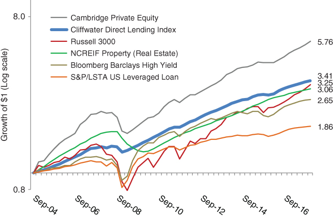
EXHIBIT 3.2 Asset class cumulative returns (growth of $1.00), September 2004 to December 2017.

Return and risk measures cover the same 13.25‐year period encompassing the CDLI and are based upon quarterly returns so that all calculations are consistent. Only US asset classes are included because the comparison is meant to gauge return and risk within a single market, without currency and country specific impacts.

In Exhibit 3.1 asset classes are grouped by type. The Russell 3000 Index, which includes large and middle market companies, represents the performance of the US public equity market. Next, three measures of investment‐grade fixed income are provided. The Merrill Lynch 0–3 Month Treasury Bill Index represents short‐term rates; the Bloomberg Barclays 3–5 Year Treasury Index represents intermediate‐term fixed income with a similar maturity as direct loans; and the Bloomberg Barclays Aggregate Bond Index represents the most popular benchmark for fixed income portfolios; it is the index most commonly used for passive fixed income investing. Two measures of traded, non‐investment‐grade credit are provided. The S&P/LSTA Leveraged Loan Index measures the performance of broadly syndicated bank loans and is the most common index currently used to benchmark direct loan and other private debt strategies. The Bloomberg Barclays High Yield Bond Index is the most common index used to benchmark high‐yield bond portfolios. Like direct lending, high‐yield bonds are non‐investment grade, but they are typically actively traded, not buy and hold, and have fixed‐, not floating‐rate coupons. Lastly, Exhibit 3.1 shows two other private asset classes in addition to the CDLI. NCREIF (National Council on Real Estate Investment Fiduciaries) measures the quarterly performance of institutional real estate equity. Its construction is very similar to that used for the CDLI. Finally, the Cambridge Associates US Private Equity Index measures performance of private partnerships that invest in private companies, not private equity companies themselves. The Cambridge Associates US Private Equity Index is net of fees while the other indices are reported gross of fees.

RETURN

The historical asset class returns shown in Exhibit 3.1 are consistent with expectations. US private equity, measured by the Cambridge Associates US Private Equity Index was the best performing asset class with a 14.1% annualized return, which was 4.8% above the Russell 3000 Index return of public US equities. The 4.8% difference compares favorably with the 3% per annum excess return for private equity over public equity targeted by most institutional investors.

Direct lending, measured by the CDLI, returned an annualized 9.7% and outperformed the other asset classes listed except for private equity, which it trailed by 4.4%. The outperformance by the Cambridge Associates US Private Equity Index should be expected because it represents capital that has less seniority than direct loans in the corporate capital structure and therefore should have a higher return. Given that the private equity returns are net of fees and the CDLI is gross of fees, the difference would be closer to 6–7% if the CDLI were adjusted for likely fees and expenses. This estimated net‐of‐fee difference in private equity and private debt returns is in line with underwriting of sponsored equity and debt financing.

The 9.7% CDLI return outperformed the NCREIF Property Index (NPI) of institutional commercial real estate equity return of 8.8% for the measurement period, which is of note because both indices have common construction methodologies and similar ASC 820 oversight in asset valuation. Also, both asset classes share the common role of stable income and lower risk within diversified institutional portfolios.

Another important comparison is between the 9.7% CDLI return and the 4.8% S&P/LSTA US Leveraged Loan Index returns. This 4.9% average yearly difference is approximately equal to the historical yield spread between the two indices and represents a reasonable expectation for a return premium for private floating‐rate non‐investment‐grade loans. Adjusted for fees, the estimated difference is closer to 3.5% because direct lending investors pay roughly 1.5% more for a direct loan portfolio compared to a portfolio of bank leveraged loans. Some early direct lending investors are benchmarking their direct lending portfolios to a 1% spread over the S&P/LSTA US Leveraged Loan Index. The historical returns in Exhibit 3.1 suggest this might be a conservative benchmark.

At first glance, the 7.6% annualized return for the Bloomberg Barclays High Yield Bond Index looks attractive compared to the 4.8% return on the S&P/LSTA US Leveraged Loan Index. However, the comparison is somewhat misleading because 7.6% return is based on fixed‐rate bonds and the 4.8% is based on floating‐rate loans. The high‐yield bond return can be adjusted for the fixed/floating difference by subtracting the spread between the Bloomberg Barclays 3–5 Year US Treasury return of 3.3% and the Merrill Lynch 0–3 Month T‐Bill return of 1.3%. The 2.0% difference is what needs to be subtracted from the 7.6% Bloomberg Barclays High Yield Bond Index return to get an equivalent floating‐rate return for high‐yield bonds equal to 5.6%, annualized, and a return that would be equivalent to buying high‐yield bonds but adding a fixed/floating interest rate swap.

Before fees, the floating‐rate credit indices returned 9.7%, 5.6%, and 4.8% for direct loans, high‐yield bonds, and leveraged loans, respectively, over the 13.25‐year measurement period. Adjusting for estimated fees equal to 2.0%, 0.5%, and 0.5% for direct loans, high‐yield bonds, and leveraged loans, respectively, after‐fee and floating‐rate equivalent returns for these three asset classes would equal 7.7%, 5.1%, and 4.3%, respectively. The 0.8% spread between public high‐yield bonds and leveraged bank loans is attributable to the subordinated credit position of most high‐yield bonds, which should entail a higher credit spread compared to leveraged bank loans.

Exhibit 3.2 provides a graphical representation of asset class returns. The three lowest returning, and lowest risk, asset classes consisting of investment‐grade fixed income are dropped for visual clarity. As in Exhibit 2.2, cumulative returns in Exhibit 3.2 are plotted on a log scale so that a constant return appears as a straight line and drawdowns are scaled by return, not dollar loss.

The strong performance for private equity (Cambridge Associates US Private Equity Index) is strikingly clear from Exhibit 3.2 with a hypothetical $1.00 invested on September 30, 2004 growing to $5.76 by December 31, 2017. In comparison to public equity (Russell 3000 Index), the performance difference is shown to be quite wide but with most of the discrepancy concentrated in the first half of the measurement period. The performance shown for the CDLI is not as strong as it is for private equity, but in a comparison with equivalent public securities, measured by the S&P/LSTA Leveraged Loan Index, the CDLI displays consistent and widening separation. The point is that private equity performance outperforms public equity over long periods of time but in spurts, partly due to valuation lags, and generally when public equity returns are more subdued. Exhibit 3.2 shows that private debt (CDLI) should produce excess return compared to public debt (S&P/LSTA Leveraged Loan Index) on a more consistent basis because both asset classes are less volatile and private debt is less vulnerable to valuation lag effects.

RISK AND MAXIMUM DRAWDOWN

Historical standard deviation of return in the second column and maximum drawdown in the fourth column of Exhibit 3.1 give investors a comparison of the volatility found in direct lending compared to the other asset classes.

Historical risk values for the public asset classes are consistent with expectations, with public equity measuring the highest at 15.1% standard deviation; non‐investment‐grade credit through bank loans and high‐yield bonds incurring slightly less risk at 10.2% and 10.7%, respectively; investment‐grade, intermediate‐maturity bonds represented by the Bloomberg Barclays Aggregate Bond Index and 3–5 Year US Treasuries measuring risk at 3.2% and 3.7%, respectively; and cash equivalents at a 0.9% risk level.

Standard deviations for private equity, private real estate, and private direct loans equal 9.9%, 5.5%, and 3.5%, respectively. Relative volatility between these three private asset classes is likely consistent with the perceived risk being taken, with private equity the highest risk and private debt the lowest risk. However, the absolute levels of risk from private assets is likely understated due to the use of fair value accounting, which results in some smoothing of asset values. This undoubtedly occurs, but it is difficult to precisely measure its impact on risk and correlation. We address this issue in more detail in Chapter 14.

Investors look at maximum drawdown as another important measure of risk. Maximum drawdown measures the cumulative, unannualized, percentage decline in value from peak value to lowest value. Maximum drawdown became an important complement to the more familiar standard deviation risk measure after the 2008–2009 global financial crisis (GFC). The standard deviation measure of risk works only if the periodic returns upon which the calculation is based are uncorrelated with each other. (They are not serially correlated and follow a random walk.) But that is not how markets behaved in 2008 and 2009. Down months followed down months in a pattern that leads a standard deviation risk measure to understate the true risk of loss. As a result, most investment professionals added the maximum drawdown calculation to their risk metrics. The maximum drawdown calculation also avoids the understatement of standard deviation risk caused by the serial correlation.

Though it occurred 10 years ago now, the near halving of stock values during the GFC hasn't been forgotten. The maximum drawdown for the Russell 3000 Index equaled −46%, transpiring over a six‐quarter period from September 30, 2007 through March 31, 2009, and gave rise to a renewed emphasis on risk management strategies. In hindsight, Treasury securities proved to be the best risk mitigator. Treasury indices, and broader investment‐grade bond indices like the Bloomberg Barclays Aggregate Bond Index, which is predominately comprised of Treasury and agency bonds and notes, lost little or no value during the GFC, earning risk‐off status among chief risk officers. However, as investment professionals discovered, the opportunity cost of holding these securities has been significant, with Treasury yields averaging less than 3%, and sometimes below 2%. Since the GFC, asset allocators have been looking for strategies or asset classes that might better balance return and risk and sit somewhere between stocks and Treasuries in the risk spectrum. The performance of direct loans suggests that it might be a good choice to fill that between role.

Make no mistake, direct loans are a risk‐on asset class, as the correlations in Exhibit 3.1 demonstrate. The correlation between the CDLI and the Russell 3000 index measures 0.68. R‐squared, the square of the correlation, equals 0.46, meaning that 46% of the volatility of the CDLI is explained by the volatility of the Russell 3000 index. In other words, direct loan returns are heavily influenced by the ups and downs of stocks.

However, direct loan fair values do not display the same high volatility as stocks. While directionally influenced by stocks, direct loan values have a Treasury‐like 3.5% standard deviation. The CDLI beta to the Russell 3000 Index, which is the product of relative standard deviation and correlation, measures 0.16 and would be considered a strong portfolio diversifier by most risk management standards.

Not surprisingly, the CDLI also experienced a drawdown as stocks declined during the GFC, but its 8% decline was far less than other risk‐on asset classes. Real estate had historically been viewed as a lower risk, equity‐oriented asset class but its 24% drawdown during the GFC changed that perception for many, though this drawdown was certainly understandable since the GFC was triggered by upheaval in the US housing market and related securities. Exhibit 3.3 provides an instructive picture of the drawdown in direct loans that began on June 30, 2008 and which can be used by potential investors for stress testing.

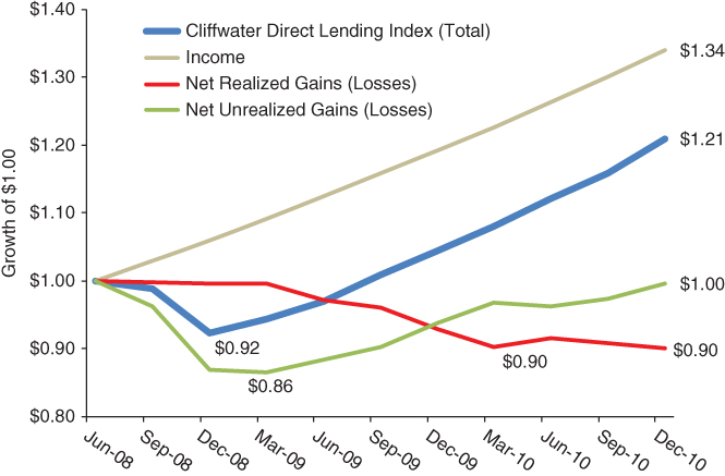
EXHIBIT 3.3 Direct lending drawdown during the global financial crisis, June 30, 2008 to December 31, 2010.

In the case of direct loans, high current interest income provides a strong buffer against losses. At the June 2008 start of the drawdown period, the current yield on the CDLI equaled 9.90% and subsequently increased during the drawdown period, reaching a 11.27% December 2008 high. Loan valuations were adjusted downward immediately in the third and fourth quarters of 2008, creating unrealized losses peaking at 14% ($0.86) on March 31, 2009. The 8% drawdown cited in Exhibit 3.1 came after six months and was a combination of current income being more than offset by the rapid downward adjustments to loan fair values. Note that realized losses did not contribute to the 8% CDLI maximum drawdown. Realized losses came gradually in subsequent quarters and totaled 10% ($0.90) when they bottomed in March 2010. The unrealized losses were replaced by realized losses until December 2010 when they were again zero ($1.00).

An important observation about the behavior of direct loans during the GFC is that the fair value accounting process worked. In fact, one could argue that the process worked too well (e.g., was too conservative). In the end, the 14% in unrealized losses imposed on direct loans in the first six months of the GFC exceeded the 10% in realized losses or actual principal impairments that ended in March 2010. If we can think of unrealized losses as loan loss reserves, those doing independent valuations on loans overestimated future impairments by 4%. In the end, the 2008 GFC was not only a stress test on direct loan performance, but also a stress test on the process used to determine loan values.