![$$\displaystyle \begin{aligned} \begin{array}{rcl}{} \min_{\mathbf{x}} f(\mathbf{x})\equiv \mathbb{E} [F(\mathbf{x};\xi)], \end{array} \end{aligned} $$](../images/487003_1_En_5_Chapter/487003_1_En_5_Chapter_TeX_Equ1.png)

- 1.
in theory, most convergence properties are studied in the forms of expectation (concentration);
- 2.
in real experiments, the algorithms are often much faster than the batch (deterministic) ones.
Because the updates access the gradient individually, the time complexity to reach a tolerable accuracy can be evaluated by the total number of calls for individual functions. Formally, we refer to it as the Incremental First-order Oracle (IFO) calls, with definition as follows:
For problem (5.2), an IFO takes an index i ∈ [n] and a point  , and returns the pair (f
i(x), ∇f
i(x)).
, and returns the pair (f
i(x), ∇f
i(x)).
As has been discussed in Chap. 2, the momentum (acceleration) technique ensures a theoretically faster convergence rate for deterministic algorithms. We might ask whether the momentum technique can accelerate stochastic algorithms. Before we answer the question, we first put our attention on the stochastic algorithms itself. What is the main challenge in analyzing the stochastic algorithms? Definitely, it is the noise of the gradients. Specifically, the variance of the noisy gradient will not go to zero through the updates, which fundamentally slows down the convergence rate. So a more involved question is to ask whether the momentum technique can reduce the negative effect of noise? Unfortunately, the existing results answer the question with “No.” The momentum technique cannot reduce the variance but instead can accumulate the noise. What really reduces the negative effect of noise is the technique called variance reduction (VR) [10]. When applying the VR technique, the algorithms are transformed to act like a deterministic algorithm and then can be further fused with momentum . Now we are able to answer our first question. The answer is towards positivity: in some cases, however, not all (e.g., when n is large), the momentum technique fused with VR ensures a provably faster rate! Besides, another effect of the momentum technique is that it can accumulate the noise. Thus one can reduce the variance together after it is aggregated by the momentum . By doing this, the mini-batch sampling size is increased, which is very helpful in distributed optimization (see Chap. 6).
- 1.
transforming the algorithm into a “near deterministic” one by VR and
- 2.
fusing the momentum trick to achieve a faster rate of convergence.
Ensure faster convergence rates (by order) when n is sufficiently small.
Ensure larger mini-batch sizes for distributed optimization.
each f i(x) is convex, which we call the individually convex (IC) case.
each f i(x) can be nonconvex but f(x) is convex, which we call the individually nonconvex (INC) case.
f(x) is nonconvex (NC).
5.1 The Individually Convex Case

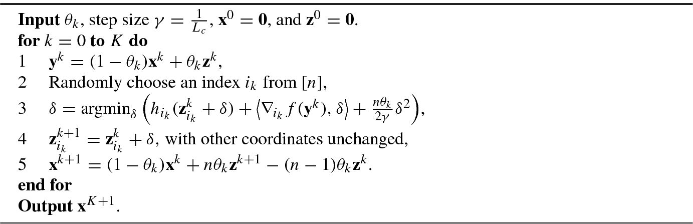
5.1.1 Accelerated Stochastic Coordinate Descent

 with
with  , and f(x) and h
i(x) are convex.
, and f(x) and h
i(x) are convex. is chosen to sufficiently reduce the objective value while keeping other coordinates fixed, reducing the per-iteration cost. More specifically, the following types of proximal subproblem are solved:
 denotes the partial gradient of f with respect to
  . Fusing with the momentum
technique, ASCD
is shown in Algorithm 5.1.
. Fusing with the momentum
technique, ASCD
is shown in Algorithm 5.1.We give the convergence result below. The proof is taken from [8].
 and for all k ≥ 0, θ
k ≥ 0 and is monotonically non-increasing, then x
k is a convex combination of z
0, ⋯ , z
k, i.e., we have
and for all k ≥ 0, θ
k ≥ 0 and is monotonically non-increasing, then x
k is a convex combination of z
0, ⋯ , z
k, i.e., we have  , where e
0,0 = 1, e
1,0 = 1 − nθ
0, e
1,1 = nθ, and for k > 1, we have
, where e
0,0 = 1, e
1,0 = 1 − nθ
0, e
1,1 = nθ, and for k > 1, we have 
 , we have

where
 denotes that the expectation is taken only on the random number i
kunder the condition thatx
kandz
kare known.
denotes that the expectation is taken only on the random number i
kunder the condition thatx
kandz
kare known.
![$$\displaystyle \begin{aligned} \begin{array}{rcl} {\mathbf{x}}^{k+1} &\displaystyle \overset{a}=&\displaystyle (1-\theta_k){\mathbf{x}}^k +\theta_k {\mathbf{z}}^k +n\theta_k ({\mathbf{z}}^{k+1}-{\mathbf{z}}^k)\\ &\displaystyle =&\displaystyle (1-\theta_k)\sum_{i=0}^k e_{k,i}{\mathbf{z}}^i +\theta_k {\mathbf{z}}^k +n\theta_k({\mathbf{z}}^{k+1}-{\mathbf{z}}^{k})\\ &\displaystyle =&\displaystyle (1-\theta_k)\sum_{i=0}^{k-1} e_{k,i}{\mathbf{z}}^i +\left[(1-\theta_k)e_{k,k}+\theta_k -n\theta_k\right]{\mathbf{z}}^k +n\theta_k {\mathbf{z}}^{k+1}, \end{array} \end{aligned} $$](../images/487003_1_En_5_Chapter/487003_1_En_5_Chapter_TeX_Equ8.png)
 uses Step 5 of Algorithm 5.1. Comparing the results, we obtain (5.5). Next, we prove that the above is a convex combination. It is easy to prove that the weights sum to 1 (by induction), 0 ≤ (1 − θ
k)e
k,j ≤ 1, and 0 ≤ nθ
k ≤ 1. So (1 − θ
k)e
k,k + θ
k − nθ
k = n(1 − θ
k)θ
k−1 + θ
k − nθ
k ≤ 1. On the other hand, we have
uses Step 5 of Algorithm 5.1. Comparing the results, we obtain (5.5). Next, we prove that the above is a convex combination. It is easy to prove that the weights sum to 1 (by induction), 0 ≤ (1 − θ
k)e
k,j ≤ 1, and 0 ≤ nθ
k ≤ 1. So (1 − θ
k)e
k,k + θ
k − nθ
k = n(1 − θ
k)θ
k−1 + θ
k − nθ
k ≤ 1. On the other hand, we have 
![$$\displaystyle \begin{aligned} \begin{aligned} &\mathbb{E}_{i_k}\hat{h}_{k+1}\\ &\quad \overset{a}= \sum_{i=0}^k e_{k+1,i} h({\mathbf{z}}^i) +\mathbb{E}_{i_k} \left[n\theta_k h({\mathbf{z}}^{k+1})\right]\\ &\quad = \sum_{i=0}^ke_{k+1,i} h({\mathbf{z}}^i) +\frac{1}{n}\sum_{i_k} n\theta_k \left(h_{i_k}({\mathbf{z}}^{k+1}_{i_k})+\sum_{j\neq i_k}h_j({\mathbf{z}}^k_j) \right)\\ &\quad = \sum_{i=0}^ke_{k+1,i} h ({\mathbf{z}}^i) +\theta_k\sum_{i_k} h_{i_k}({\mathbf{z}}^{k+1}_{i_k})+(n-1)\theta_k h({\mathbf{z}}^k) \\ &\quad \overset{b}= \sum_{i=0}^{k-1} e_{k+1,i} h({\mathbf{z}}^i) +[n(1-\theta_k)\theta_{k-1}+\theta_k-n\theta_k]h({\mathbf{z}}^k)+(n-1)\theta_kh({\mathbf{z}}^k) \\ &\qquad +\theta_k\sum_{i_k} h_{i_k}({\mathbf{z}}^{k+1}_{i_k})\\ &\quad = \sum_{i=0}^{k-1}e_{k+1,i} h({\mathbf{z}}^i)+n(1-\theta_k)\theta_{k-1}h({\mathbf{z}}^k)+\theta_k\sum_{i_k} h_{i_k}({\mathbf{z}}^{k+1}_{i_k})\\ \end{aligned} \end{aligned}$$](../images/487003_1_En_5_Chapter/487003_1_En_5_Chapter_TeX_Equa.png)

where in  we use e
k+1,k+1 = nθ
k, in
we use e
k+1,k+1 = nθ
k, in  we use e
k+1,k = n(1 − θ
k)θ
k−1 + θ
k − nθ
k, and in
we use e
k+1,k = n(1 − θ
k)θ
k−1 + θ
k − nθ
k, and in  we use e
k+1,i = (1 − θ
k)e
k,i for i ≤ k − 1, and e
k,k = nθ
k−1. □
we use e
k+1,i = (1 − θ
k)e
k,i for i ≤ k − 1, and e
k,k = nθ
k−1. □

![$$\displaystyle \begin{aligned} \begin{array}{rcl}{} &\displaystyle &\displaystyle \frac{\mathbb{E} [F({\mathbf{x}}^{K+1})] -F({\mathbf{x}}^*)}{\theta_K^2} +\frac{n^2L_c}{2}\mathbb{E}\|{\mathbf{z}}^{K+1} -{\mathbf{x}}^* \|{}^2\\ &\displaystyle &\displaystyle \quad \leq\frac{F({\mathbf{x}}^0)-F({\mathbf{x}}^*)}{\theta_{-1}^2} +\frac{n^2L_c}{2}\|{\mathbf{z}}^0 -{\mathbf{x}}^*\|{}^2. \end{array} \end{aligned} $$](../images/487003_1_En_5_Chapter/487003_1_En_5_Chapter_TeX_Equ10.png)
 which is denoted as θ instead, we have
 ![$$\displaystyle \begin{aligned} \begin{array}{rcl}{} &\displaystyle &\displaystyle \mathbb{E} [F({\mathbf{x}}^{K+1})] -F({\mathbf{x}}^*)\\ &\displaystyle &\displaystyle \quad \leq (1-\theta)^{K+1} \left(F({\mathbf{x}}^0) -F({\mathbf{x}}^*)+ \frac{n^2\theta^2L_c+n\theta\mu}{2}\left\|{\mathbf{z}}^{0} -{\mathbf{x}}^* \right\|{}^2 \right). \end{array} \end{aligned} $$](../images/487003_1_En_5_Chapter/487003_1_En_5_Chapter_TeX_Equ11.png)
 in Step 4, we have
 . By Steps 1 and 5, we have


 uses Proposition A.7, in
  we use (5.11), in
  we insert
  , and
, and  uses
uses  .
.


 uses the convexity of f. Taking expectation on (5.12) and adding (5.14) and (5.15), we have
 we use (5.10).
 (μ ≥ 0), we have
![$$\displaystyle \begin{aligned} \begin{array}{rcl}{} \mathbb{E}_{i_k} \left\|{\mathbf{z}}^{k+1}-{\mathbf{x}}^* \right \|{}^2 &\displaystyle =&\displaystyle \frac{1}{n}\sum_{i_k=1}^n\left[ \left ({\mathbf{z}}^{k+1}_{i_k}-{\mathbf{x}}^*_{i_k} \right)^2 + \sum_{j\neq i_k} \left({\mathbf{z}}^{k+1}_{j}-{\mathbf{x}}^*_{j} \right)^2 \right] \\ &\displaystyle \overset{a}=&\displaystyle \frac{1}{n}\sum_{i_k=1}^n\left[ \left ({\mathbf{z}}^{k+1}_{i_k}-{\mathbf{x}}^*_{i_k} \right)^2 + \sum_{j\neq i_k} \left({\mathbf{z}}^{k}_{j}-{\mathbf{x}}^*_{j} \right)^2 \right] \\ &\displaystyle =&\displaystyle \frac{1}{n}\sum_{i_k=1}^n\left({\mathbf{z}}^{k+1}_{i_k}-{\mathbf{x}}^*_{i_k} \right)^2+\frac{n-1}{n} \left\|{\mathbf{z}}^{k}-{\mathbf{x}}^*\right \|{}^2, \end{array} \end{aligned} $$](../images/487003_1_En_5_Chapter/487003_1_En_5_Chapter_TeX_Equ21.png)
 we use
  , j ≠ i
k. Similar to (5.17), we also have
, j ≠ i
k. Similar to (5.17), we also have ![$$\displaystyle \begin{aligned} \begin{array}{rcl} \mathbb{E}_{i_k}\left \|{\mathbf{x}}^{k+1}-{\mathbf{y}}^k \right\|{}^2 &\displaystyle =&\displaystyle \frac{1}{n}\sum_{i_k=1}^n\left[ \left({\mathbf{x}}^{k+1}_{i_k}-{\mathbf{y}}^k_{i_k} \right)^2 + \sum_{j\neq i_k} \left({\mathbf{x}}^{k+1}_{j}-{\mathbf{y}}^k_{j} \right)^2 \right] \\ &\displaystyle \overset{a}=&\displaystyle \frac{1}{n}\sum_{i_k=1}^n\left({\mathbf{x}}^{k+1}_{i_k}-{\mathbf{y}}^k_{i_k}\right)^2, \end{array} \end{aligned} $$](../images/487003_1_En_5_Chapter/487003_1_En_5_Chapter_TeX_Equ22.png)
 we use
  , j ≠ i
k. Then we obtain
, j ≠ i
k. Then we obtain 
 uses (5.16),
  uses (5.17), and
  uses Lemma 5.1.

 we use
  when k ≥−1. Taking full expectation, we have
 we use
  . Then using the convexity of h(x) and that x
k+1 is a convex combination of z
0, ⋯ , z
k+1, we have
. Then using the convexity of h(x) and that x
k+1 is a convex combination of z
0, ⋯ , z
k+1, we have 
 uses Lemma 5.1. So we obtain (5.7).


Taking full expectation, expanding the result to k = 0, then using  (see (5.19)),
  , and ∥z
k+1 −x
∗∥2 ≥ 0, we obtain (5.8). □
, and ∥z
k+1 −x
∗∥2 ≥ 0, we obtain (5.8). □

 , i = 1, ⋯ , n, are loss functions over training samples. Lots of machine learning problems can be formulated as (5.20), such as linear SVM, ridge regression, and logistic regression. For ASCD
, we can solve (5.20) via its dual problem
:
, i = 1, ⋯ , n, are loss functions over training samples. Lots of machine learning problems can be formulated as (5.20), such as linear SVM, ridge regression, and logistic regression. For ASCD
, we can solve (5.20) via its dual problem
: 
 is the conjugate function
(Definition A.21) of ϕ
i(⋅) and A = [A
1, ⋯ , A
n]. Then (5.21) can be solved by Algorithm 5.1.
is the conjugate function
(Definition A.21) of ϕ
i(⋅) and A = [A
1, ⋯ , A
n]. Then (5.21) can be solved by Algorithm 5.1.5.1.2 Background for Variance Reduction Methods
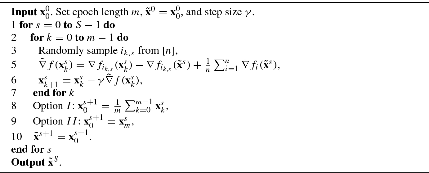
For stochastic gradient descent , due to the nonzero variance of the gradient, using a constant step size cannot guarantee the convergence of algorithms. Instead, it only guarantees a sublinear convergence rate on the strongly convex and L-smooth objective functions. For finite-sum objective functions, the way to solve the problem is called variance reduction (VR) [10] which reduces the variance to zero through the updates. The convergence rate can be accelerated to be linear for strongly convex and L-smooth objective functions. The first VR method might be SAG [17], which uses the sum of the latest individual gradients as an estimator. It requires O(nd) memory storage and uses a biased gradient estimator. SDCA [18] also achieves a linear convergence rate. In the primal space, the algorithm is known as MISO [13], which is a majorization-minimization VR algorithm. SVRG [10] is a follow-up work of SAG [17] which reduces the memory costs to O(d) and uses an unbiased gradient estimator. The main technique of SVRG [10] is frequently pre-storing a snapshot vector and bounding the variance by the distance from the snapshot vector and the latest variable. Later, SAGA [6] improves SAG by using an unbiased updates via the technique of SVRG [10].


 . In other words, by setting
  and
and  , the IFO
calls (Definition 5.1) to achieve an 𝜖-accuracy solution is
, the IFO
calls (Definition 5.1) to achieve an 𝜖-accuracy solution is  . If each f
i(x) is L-smooth (but might be nonconvex) and f(x) is μ-strongly convex, by setting
. If each f
i(x) is L-smooth (but might be nonconvex) and f(x) is μ-strongly convex, by setting  and m = −ln
−1(1 − ημ∕2) ∼ O(η
−1μ
−1), we have
and m = −ln
−1(1 − ημ∕2) ∼ O(η
−1μ
−1), we have 
In other words, the IFO
calls to achieve an 𝜖- accuracy solution is  .
.
The proof is mainly taken from [10] and [4].
 denote the expectation taken only on the random number i
k,s conditioned on
denote the expectation taken only on the random number i
k,s conditioned on  . Then we have
 is an unbiased estimator of
  . Then
 we use ∥a −b∥2 ≤ 2∥a∥2 + 2∥b∥2 and in
  we use Proposition A.2.
 and y = x
∗ in (5.26) and summing the result with i = 1 to n, we have
and y = x
∗ in (5.26) and summing the result with i = 1 to n, we have 

![$$\displaystyle \begin{aligned} \begin{array}{rcl}{} \mathbb{E}_k\left\| \tilde{\nabla} f({\mathbf{x}}^s_k) \right\|{}^2\leq 4L \left[ (f({\mathbf{x}}^s_k) - f({\mathbf{x}}^*)) + (f(\tilde{\mathbf{x}}^s) - f({\mathbf{x}}^*))\right]. \end{array} \end{aligned} $$](../images/487003_1_En_5_Chapter/487003_1_En_5_Chapter_TeX_Equ39.png)
![$$\displaystyle \begin{aligned} &\mathbb{E}_k\|{\mathbf{x}}^s_{k+1} - {\mathbf{x}}^* \|{}^2 \\ &\quad = \|{\mathbf{x}}^s_{k} - {\mathbf{x}}^* \|{}^2+ 2\mathbb{E}_k\left\langle {\mathbf{x}}^s_{k+1} - {\mathbf{x}}^s_{k} , {\mathbf{x}}^s_{k} - {\mathbf{x}}^* \right\rangle +\mathbb{E}_k \|{\mathbf{x}}^s_{k+1} - {\mathbf{x}}^s_{k}\|{}^2\\ &\quad =\|{\mathbf{x}}^s_{k} - {\mathbf{x}}^* \|{}^2 - 2\eta\mathbb{E}_k\left\langle \tilde{\nabla} f({\mathbf{x}}_k^s), {\mathbf{x}}_k^s - {\mathbf{x}}^*\right\rangle + \eta^2\mathbb{E}_k\| \tilde{\nabla} f({\mathbf{x}}^s_k) \|{}^2\\ &\quad \overset{a} \leq \|{\mathbf{x}}^s_{k} - {\mathbf{x}}^* \|{}^2 - 2\eta \left\langle \nabla f({\mathbf{x}}^s_k), {\mathbf{x}}_k^s - {\mathbf{x}}^* \right\rangle \\ &\qquad + 4L\eta^2\left[ (f({\mathbf{x}}_k^s) - f({\mathbf{x}}^*))+(f(\tilde{\mathbf{x}}^s) - f({\mathbf{x}}^*))\right]\\ &\quad \leq\|{\mathbf{x}}^s_{k} - {\mathbf{x}}^* \|{}^2 - 2 \eta (1 - 2 L \eta)[ f({\mathbf{x}}^{s}_k) - f({\mathbf{x}}^*)] + 4L\eta^2[f(\tilde{\mathbf{x}}^s) - f({\mathbf{x}}^*)], \end{aligned} $$](../images/487003_1_En_5_Chapter/487003_1_En_5_Chapter_TeX_Equ40.png)


 uses Option I of Algorithm 5.2 and
  is by telescoping (5.30). Using
  , we can obtain (5.23).


 and
and  use (5.24) and
  uses Proposition A.2.
 . Substituting (5.34) into (5.33) after taking expectation on i
k, we have
. Substituting (5.34) into (5.33) after taking expectation on i
k, we have 

 . Now we consider k + 1. We consider Option II in Algorithm 5.2 and have
 uses k ≤ m = −ln−1(1 − ημ∕2). Then we have
 uses
uses  .
.Taking full expectation on (5.35) and substituting (5.36) into it, we can obtain that  . □
. □
5.1.3 Accelerated Stochastic Variance Reduction Method
With the VR
technique, we can fuse the momentum
technique to achieve a faster rate. We show that the convergence rate can be improved to  in the IC case, where
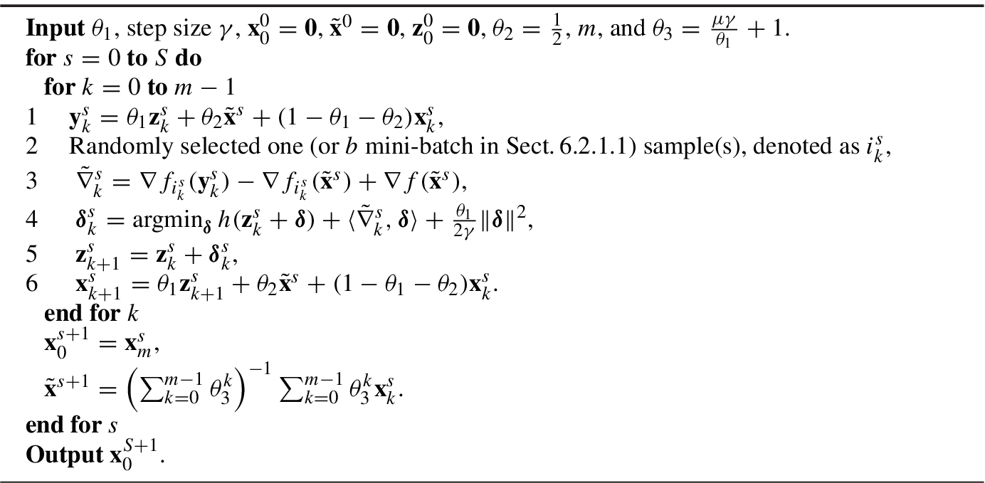
  . We introduce Katyusha
[1], which is the first truly accelerated stochastic algorithm. The main technique in Katyusha
[1] is introducing a “negative momentum
” which restricts the extrapolation term to be not far from
. We introduce Katyusha
[1], which is the first truly accelerated stochastic algorithm. The main technique in Katyusha
[1] is introducing a “negative momentum
” which restricts the extrapolation term to be not far from  , the snapshot vector introduced by SVRG
[10]. The algorithm is shown in Algorithm 5.3.
, the snapshot vector introduced by SVRG
[10]. The algorithm is shown in Algorithm 5.3.
The proof is taken from [1]. We have the following lemma to bound the variance:
 , with each f
i with i ∈ [n] being convex and L-smooth. For any u and
, with each f
i with i ∈ [n] being convex and L-smooth. For any u and  , defining

where the expectation is taken on the random number k under the condition thatuand
 are known.


 . For Algorithm 5.3, if the step size
  ,
,  ,
,  , and m = n, we have
 ![$$\displaystyle \begin{aligned} \begin{array}{rcl} F(\tilde{\mathbf{x}}^{S+1})-F({\mathbf{x}}^*) \leq \theta_3^{-Sn}\left[\frac{1}{4n\gamma}\|{\mathbf{z}}^0_0-{\mathbf{x}}^* \|{}^2 + \left(1+\frac{1}{n}\right) \left(F({\mathbf{x}}^0_0)-F({\mathbf{x}}^*) \right) \right]. \end{array} \end{aligned} $$](../images/487003_1_En_5_Chapter/487003_1_En_5_Chapter_TeX_Equ54.png)
 and
and  , we have


 in Step 4 of Algorithm 5.3, there exists
  satisfying


 we add and subtract the term
  and
and  uses the equality (5.41).
 to denote that expectation is taken on the random number
  (step k and epoch s) under the condition that
  is known, in
  we use the Cauchy–Schwartz inequality, and
  uses (5.37). C
3 is an absolute constant determined later.
uses (5.37). C
3 is an absolute constant determined later.

 . Setting a = 1 − θ
1 − θ
2, we have
. Setting a = 1 − θ
1 − θ
2, we have 
 uses Step 1 of Algorithm 5.3.
 we use
  and that
  is constant, because the expectation is taken only on the random number i
k,s, and in inequality
is constant, because the expectation is taken only on the random number i
k,s, and in inequality  we use the convexity of f(⋅) and so for any vector u,
 , we have
 uses (5.46). Adding (5.47) and (5.44), we obtain that
 we set
  . For the last term of (5.48), we have
 we use
  and the convexity of h(⋅). Substituting (5.49) into (5.48), we obtain
 and
and  . Taking expectation on (5.50) for the first k − 1 iterations, then multiplying it with
  , and telescoping the results with k from 0 to m − 1, we have
 ![$$\displaystyle \begin{aligned} &\sum_{k=1}^{m} \theta_3^{k-1} \left(F({\mathbf{x}}^s_{k})-F({\mathbf{x}}^*) \right) - a\sum_{k=0}^{m-1} \theta_3^k \left(F({\mathbf{x}}^s_{k})-F({\mathbf{x}}^*) \right)\\ &\quad - \theta_2\sum_{k=0}^{m-1} \left[\theta_3^k \left(F(\tilde{\mathbf{x}}^s)-F({\mathbf{x}}^*) \right)\right] + \frac{\theta_3^{m}}{2\gamma}\left\| \theta_1{\mathbf{z}}^s_m- \theta_1{\mathbf{x}}^*\right\|{}^2 \leq \frac{1}{2\gamma}\left\| \theta_1 {\mathbf{z}}^s_0 - \theta_1{\mathbf{x}}^*\right\|{}^2. \end{aligned} $$](../images/487003_1_En_5_Chapter/487003_1_En_5_Chapter_TeX_Equ69.png)
![$$\displaystyle \begin{aligned} \begin{array}{rcl} &\displaystyle &\displaystyle [\theta_1+\theta_{2} -(1-1/\theta_3)]\sum_{k=1}^{m} \theta_3^k \left(F({\mathbf{x}}^s_{k})-F({\mathbf{x}}^*) \right) + \theta_3 ^ma \left(F({\mathbf{x}}^s_{m})-F({\mathbf{x}}^*)\right)\\ &\displaystyle &\displaystyle \quad +\frac{\theta_3^{m}}{2\gamma}\left\| \theta_1{\mathbf{z}}^s_m- \theta_1{\mathbf{x}}^*\right\|{}^2\\ &\displaystyle &\displaystyle \qquad \leq \theta_2\sum_{k=0}^{m-1} \left[\theta_3^k \left(F(\tilde{\mathbf{x}}^s)-F({\mathbf{x}}^*) \right)\right] +a \left(F({\mathbf{x}}^s_{0}){-}F({\mathbf{x}}^*)\right)+ \frac{1}{2\gamma}\left\| \theta_1 {\mathbf{z}}^s_0 {-} \theta_1{\mathbf{x}}^*\right\|{}^2. \end{array} \end{aligned} $$](../images/487003_1_En_5_Chapter/487003_1_En_5_Chapter_TeX_Equ70.png)
 , we have
 ![$$\displaystyle \begin{aligned} & [\theta_1+\theta_{2} -(1-1/\theta_3)]\theta_3 \left(\sum_{k=0}^{m-1} \theta_3^k\right) \left(F(\tilde{\mathbf{x}}^{s+1})-F({\mathbf{x}}^*) \right) + \theta_3 ^ma \left(F({\mathbf{x}}^s_{m})-F({\mathbf{x}}^*)\right)\\ &\quad +\frac{\theta_3^{m}}{2\gamma}\left\| \theta_1{\mathbf{z}}^s_m- \theta_1{\mathbf{x}}^*\right\|{}^2\\ &\qquad \leq \theta_2\left(\sum_{k=0}^{m-1} \theta_3^k\right) \left(F(\tilde{\mathbf{x}}^s)-F({\mathbf{x}}^*) \right) +a \left(F({\mathbf{x}}^s_{0})-F({\mathbf{x}}^*)\right)\\ &\qquad \quad + \frac{1}{2\gamma}\left\| \theta_1 {\mathbf{z}}^s_0 - \theta_1{\mathbf{x}}^*\right\|{}^2.{} \end{aligned} $$](../images/487003_1_En_5_Chapter/487003_1_En_5_Chapter_TeX_Equ71.png)
![$$\displaystyle \begin{aligned} \begin{array}{rcl}{} &\displaystyle &\displaystyle \theta_2 \Big(\theta_3^{m-1}-1\Big)+ (1-1/\theta_3) \\ &\displaystyle &\displaystyle \quad \leq\frac{1}{2}\left[ \left(1+ \frac{1}{3}\sqrt{\frac{\mu}{nL}}\right)^{m-1}-1 \right] + \frac{\frac{1}{3}\sqrt{\frac{\mu}{nL}}}{\theta_3}\\ &\displaystyle &\displaystyle \quad \overset{a}\leq \frac{1}{2}\frac{1}{2} \sqrt{\frac{n\mu}{L}} +\frac{\frac{1}{3}\sqrt{\frac{\mu}{nL}}}{\theta_3}\overset{b}{\leq}\frac{7}{12}\sqrt{\frac{n\mu}{L}} \leq \theta_1, \end{array} \end{aligned} $$](../images/487003_1_En_5_Chapter/487003_1_En_5_Chapter_TeX_Equ72.png)
 we use μn ≤ L∕4 < L, m − 1 = n − 1 ≤ n, and the fact that
 we use θ
3n ≥ θ
3 ≥ 1. To prove (5.54), we can use Taylor expansion at point x = 0 to obtain
we use θ
3n ≥ θ
3 ≥ 1. To prove (5.54), we can use Taylor expansion at point x = 0 to obtain 


![$$\displaystyle \begin{aligned} \begin{array}{rcl} &\displaystyle &\displaystyle \theta_2 \left(\sum_{k=0}^{m-1} \theta_3^k \right)\left(F(\tilde{\mathbf{x}}^{S+1})-F({\mathbf{x}}^*) \right) + (1-\theta_1-\theta_2) \left(F({\mathbf{x}}^S_{m})-F({\mathbf{x}}^*)\right)\\ &\displaystyle &\displaystyle \quad + \frac{\theta_1^2}{2\gamma}\left\|{\mathbf{z}}^{S+1}_0 - {\mathbf{x}}^*\right\|{}^2\\ &\displaystyle &\displaystyle \qquad \leq \theta_3^{-Sm}\left\{\left[\theta_2\left(\sum_{k=0}^{m-1} \theta_3^k\right) + (1-\theta_1-\theta_2)\right] \left(F({\mathbf{x}}^0_0)-F({\mathbf{x}}^*) \right) \right.\\ &\displaystyle &\displaystyle \qquad \quad \left. +\frac{\theta_1^2}{2\gamma}\left\|{\mathbf{z}}^0_0-{\mathbf{x}}^* \right\|{}^2 \right\}. \end{array} \end{aligned} $$](../images/487003_1_En_5_Chapter/487003_1_En_5_Chapter_TeX_Equ76.png)


![$$\displaystyle \begin{aligned} \begin{array}{rcl} F(\tilde{\mathbf{x}}^{S+1})-F({\mathbf{x}}^*) \leq \theta_3^{-Sn} \left[ \left(1+\frac{1}{n}\right) \left(F({\mathbf{x}}^0_0)-F({\mathbf{x}}^*) \right) +\frac{1}{4n\gamma}\left\|{\mathbf{z}}^0_0-{\mathbf{x}}^* \right\|{}^2 \right]. \end{array} \end{aligned} $$](../images/487003_1_En_5_Chapter/487003_1_En_5_Chapter_TeX_Equ77.png)
5.1.4 Black-Box Acceleration
- 1.
The black-box methods make acceleration easier, because we only need to concern the method to solve subproblems. In most time, the subproblems have a good condition number and so are easy to be solved. Specifically, for general problem of (5.3), the subproblems can be solved by arbitrary vanilla VR methods. For specific forms of (5.3), one is allowed to design appropriate methods according to the characteristic of functions to solve them without considering acceleration techniques.
- 2.
The black-box methods make the acceleration technique more general. For different properties of objectives, no matter strongly convex or not and smooth or not, the black-box methods are able to give a universal accelerated algorithm.
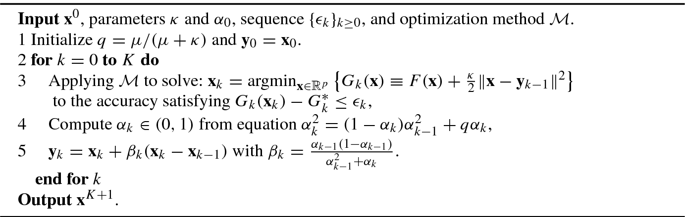
The first stochastic black-box acceleration
might be Acc-SDCA
[19]. Its convergence rate for the IC case is  . Later, Lin et al. proposed a generic acceleration, called Catalyst
[12], which achieved a convergence rate
. Later, Lin et al. proposed a generic acceleration, called Catalyst
[12], which achieved a convergence rate  , outperforming Acc-SDCA
by a factor of
, outperforming Acc-SDCA
by a factor of  . Allen-Zhu et al. [2] designed a black-box acceleration
by gradually decreasing the condition number of the subproblem, achieving
. Allen-Zhu et al. [2] designed a black-box acceleration
by gradually decreasing the condition number of the subproblem, achieving  faster rate than Catalyst
[12] on some general objective functions. In the following, we introduce Catalyst
[12] as an example. The algorithm of Catalyst
is shown in Algorithm 5.4. The main theorem for Algorithm 5.4 is as follows:
faster rate than Catalyst
[12] on some general objective functions. In the following, we introduce Catalyst
[12] as an example. The algorithm of Catalyst
is shown in Algorithm 5.4. The main theorem for Algorithm 5.4 is as follows:


We leave the proof to Sect. 5.2 and first introduce how to use it to obtain an accelerated algorithm. We have the following theorem:
For (5.3), assume that each f
i(x) is convex and L-smooth and h(x) is μ-strongly convex satisfying μ ≤ L∕n.
1 For Algorithm 5.4, if setting  and solving Step 3 by SVRG
[
10], then one can obtain an 𝜖-accuracy solution satisfying F(x) − F(x
∗) ≤ 𝜖 with IFO
calls of
and solving Step 3 by SVRG
[
10], then one can obtain an 𝜖-accuracy solution satisfying F(x) − F(x
∗) ≤ 𝜖 with IFO
calls of  .
.
The subproblem in Step 3 is  -strongly convex and
  -smooth. From Theorem 5.2, applying SVRG
to solve the subproblem needs
-smooth. From Theorem 5.2, applying SVRG
to solve the subproblem needs  IFOs
. So the total complexity is
IFOs
. So the total complexity is 
 . □
. □
The black-box algorithms, e.g., Catalyst
[12], are proposed earlier than Katyusha
[1], discussed in Sect. 5.1.3. From the convergence results, Catalyst
[12] is  times lower than Katyusha
[1]. However, the black-box algorithms are more flexible and easier to obtain an accelerated rate. For example, in the next section we apply Catalyst
to the INC case.
times lower than Katyusha
[1]. However, the black-box algorithms are more flexible and easier to obtain an accelerated rate. For example, in the next section we apply Catalyst
to the INC case.
5.2 The Individually Nonconvex Case
In this section, we consider solving (5.3) by allowing nonconvexity of f i(x) but f(x), the sum of f i(x), is still convex. One important application of it is principal component analysis [9]. It is also the core technique to obtain faster rate in the NC case.
Notice that the convexity of f(x) guarantees an achievable global minimum of (5.3). As shown in Theorem 5.2, to reach a minimizer of F(x) − F
∗≤ 𝜖, vanilla SVRG
needs IFO
calls of  . We will show that the convergence rate can be improved to be
  by acceleration. Compared with the computation costs in the IC case, the costs of NC cases are Ω(n
1∕4) times larger, which is caused by the nonconvexity of individuals. We still use Catalyst
[12] to obtain the result. We first prove Theorem 5.4 in the context of INC. The proof is directly taken from [12], which is based on the estimate sequence in [14] (see Sect. 2.1) and further takes the error of inexact solver into account.
by acceleration. Compared with the computation costs in the IC case, the costs of NC cases are Ω(n
1∕4) times larger, which is caused by the nonconvexity of individuals. We still use Catalyst
[12] to obtain the result. We first prove Theorem 5.4 in the context of INC. The proof is directly taken from [12], which is based on the estimate sequence in [14] (see Sect. 2.1) and further takes the error of inexact solver into account.
- 1.
 ;
; - 2.For k ≥ 0,
![$$\displaystyle \begin{aligned}\phi_{k+1}(\mathbf{x}) &= (1-\alpha_{k})\phi_{k}(\mathbf{x}) +\alpha_{k}\left[F({\mathbf{x}}_{k+1})+\left\langle\kappa ({\mathbf{y}}_{k} - {\mathbf{x}}_{k+1}), \mathbf{x} - {\mathbf{x}}_{k+1} \right\rangle\right] \\ &\quad +\frac{\mu}{2}\|\mathbf{x} - {\mathbf{x}}_{k+1} \|{}^2,\end{aligned} $$](../images/487003_1_En_5_Chapter/487003_1_En_5_Chapter_TeX_Equh.png)

 and v
0 = x
0 when k = 0, and γ
k, v
k, and
and v
0 = x
0 when k = 0, and γ
k, v
k, and  satisfy:
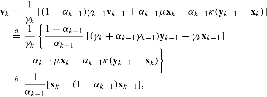
![$$\displaystyle \begin{aligned} {\mathbf{v}}_k &= \frac{1}{\gamma_k}\left[ (1 - \alpha_{k-1})\gamma_{k-1}{\mathbf{v}}_{k-1} +\alpha_{k-1}\mu {\mathbf{x}}_k- \alpha_{k-1}\kappa({\mathbf{y}}_{k-1}-{\mathbf{x}}_k) \right],{} \end{aligned} $$](../images/487003_1_En_5_Chapter/487003_1_En_5_Chapter_TeX_Equ80.png)

![$$\displaystyle \begin{aligned} \begin{array}{rcl} \begin{aligned} &\displaystyle \phi_k^* +\frac{\gamma_k}{2}\| \mathbf{x}-{\mathbf{v}}_k\|{}^2\\ &\displaystyle \quad = (1-\alpha_{k-1})\phi_{k-1}(\mathbf{x})\\ &\displaystyle \qquad +\alpha_{k-1}\left(F({\mathbf{x}}_k)+\left\langle\kappa ({\mathbf{y}}_{k-1} - {\mathbf{x}}_k), \mathbf{x} - {\mathbf{x}}_k \right\rangle] +\frac{\mu}{2}\|\mathbf{x} - {\mathbf{x}}_k \|{}^2\right). \end{aligned} \end{array} \end{aligned} $$](../images/487003_1_En_5_Chapter/487003_1_En_5_Chapter_TeX_Equ82.png)


 , we can set x = x
k in (5.59) and obtain:
, we can set x = x
k in (5.59) and obtain: 


 is the optimal solution in Step 3 of Algorithm 5.4. By the (μ + κ)-strongly convexity of G
k(x), we have
is the optimal solution in Step 3 of Algorithm 5.4. By the (μ + κ)-strongly convexity of G
k(x), we have 

 we use that G
k(x
k) is an 𝜖-accuracy solution of Step 3.
we use that G
k(x
k) is an 𝜖-accuracy solution of Step 3. . Suppose that for k − 1 with k ≥ 1, (5.60) is right, i.e.,
  . Then
 uses (5.61). Then from (5.58), we have
 uses (5.62) and
  uses (5.56).
![$$\displaystyle \begin{aligned} \begin{array}{rcl} \gamma_0 &\displaystyle =&\displaystyle \frac{\alpha_0[(\kappa+\mu)\alpha_0 -\mu]}{1 - \alpha_0},\\ \gamma_k &\displaystyle =&\displaystyle (\kappa +\mu)\alpha_{k-1}^2,\quad k\geq 1.\quad {} \end{array} \end{aligned} $$](../images/487003_1_En_5_Chapter/487003_1_En_5_Chapter_TeX_Equ91.png)

 uses (5.63) and in
  we use
 and
and  use (5.56) and
  uses (5.64).
Plugging (5.66) into (5.63) with k − 1 being replaced by k, we obtain (5.65).
 , we can have
![$$\displaystyle \begin{aligned} \begin{array}{rcl} \phi_k({\mathbf{x}}^*) &\displaystyle =&\displaystyle (1-\alpha_{k-1})\phi_{k-1}({\mathbf{x}}^*)\\ &\displaystyle &\displaystyle +\alpha_{k-1}\left(F({\mathbf{x}}_k)+\left\langle\kappa({\mathbf{y}}_{k-1}-{\mathbf{x}}_k), {\mathbf{x}}^* - {\mathbf{x}}_k\right\rangle +\frac{\mu}{2}\left\|{\mathbf{x}}^* - {\mathbf{x}}_k\right\|{}^2 \right)\\ &\displaystyle \overset{a}{\leq}&\displaystyle (1-\alpha_{k-1})\phi_{k-1}({\mathbf{x}}^*)\\ &\displaystyle &\displaystyle + \alpha_{k-1}\left[F({\mathbf{x}}^*)+ \epsilon_k -(\kappa+\mu)\left\langle {\mathbf{x}}_k - {\mathbf{x}}_k^*, {\mathbf{x}}^* - {\mathbf{x}}_k \right\rangle\right], \end{array} \end{aligned} $$](../images/487003_1_En_5_Chapter/487003_1_En_5_Chapter_TeX_Equ96.png)
 uses (5.61). Rearranging terms and using the definition of
  , we have
 we use
 uses (5.66),
  uses (A.10), and
  uses (5.64).

 uses (5.60). So we obtain (5.67).


![$$\displaystyle \begin{aligned} \begin{array}{rcl} &\displaystyle &\displaystyle \sqrt{S_k} + 2\sum_{i=1}^k\sqrt{\frac{\epsilon_i}{\lambda_i}}\\ &\displaystyle &\displaystyle \quad =\sqrt{F({\mathbf{x}}_0) - F^* + \frac{\gamma_0}{2}\|{\mathbf{x}}_0 - {\mathbf{x}}_*\|{}^2 + \sum_{i=1}^k\frac{\epsilon_i}{\lambda_i}} + 2\sum_{i=1}^k\sqrt{\frac{\epsilon_i}{\lambda_i}}\\ &\displaystyle &\displaystyle \quad \leq\sqrt{ F({\mathbf{x}}_0) - F^* + \frac{\gamma_0}{2}\|{\mathbf{x}}_0 - {\mathbf{x}}_*\|{}^2} + 3\sum_{i=1}^k\sqrt{\frac{\epsilon_i}{\lambda_i}}\\ &\displaystyle &\displaystyle \quad \leq\sqrt{ 2 (F({\mathbf{x}}_0) - F^*) } + 3\sum_{i=1}^k\sqrt{\frac{\epsilon_i}{\lambda_i}}\\ &\displaystyle &\displaystyle \quad =\sqrt{ 2 (F({\mathbf{x}}_0) - F^*) } \left[ 1+ \sum_{i=1}^k\left( \sqrt{\frac{1-\rho}{1-\sqrt{q}}} \right)^i\right]\\ &\displaystyle &\displaystyle \quad = \sqrt{ 2 (F({\mathbf{x}}_0) - F^*) } \frac{\eta^{k+1}-1}{\eta - 1}\\ &\displaystyle &\displaystyle \quad \leq \sqrt{ 2 (F({\mathbf{x}}_0) - F^*) } \frac{\eta^{k+1}}{\eta - 1}, \end{array} \end{aligned} $$](../images/487003_1_En_5_Chapter/487003_1_En_5_Chapter_TeX_Equ102.png)


With a special setting of the parameters for Algorithm 5.4, we are able to give the convergence result for the INC case.


5.3 The Nonconvex Case
In this section, we consider a hard case when f(x) is nonconvex. We only consider the problem where h(x) = 0 and focus on the IFO
complexity to achieve an approximate first-order stationary point satisfying ∥∇f(x)∥≤ 𝜖. In the IC case, SVRG
[10] has already achieved nearly optimal rate (ignoring some constants) when n is sufficiently large ( ). However, for the NC case SVRG
is not the optimal. We will introduce SPIDER
[7] which can find an approximate first-order stationary point in an optimal (ignoring some constants)
). However, for the NC case SVRG
is not the optimal. We will introduce SPIDER
[7] which can find an approximate first-order stationary point in an optimal (ignoring some constants)  rate. Next, we will show that if further assume that the objective function has Lipschitz continuous Hessians, the momentum
technique can ensure a faster rate when n is much smaller than κ = L∕μ.
rate. Next, we will show that if further assume that the objective function has Lipschitz continuous Hessians, the momentum
technique can ensure a faster rate when n is much smaller than κ = L∕μ.
5.3.1 SPIDER
 and we want to dynamically track
  for k = 0, 1, ⋯ , K. Further assume that we have an initial estimate
  and an unbiased estimate
  of
of  such that for each k = 1, ⋯ , K,
 ![$$\displaystyle \begin{aligned} \mathbb{E}\left[ \boldsymbol{\xi} _k ( \hat{\mathbf{x}}_{0:k}) \mid \hat{\mathbf{x}}_{0:k} \right] = Q(\hat{\mathbf{x}}^k ) - Q(\hat{\mathbf{x}}^{k-1} ) . \end{aligned}$$](../images/487003_1_En_5_Chapter/487003_1_En_5_Chapter_TeX_Equj.png)

 the Stochastic Path-Integrated Differential Estimator
, or SPIDER for brevity. We have
the Stochastic Path-Integrated Differential Estimator
, or SPIDER for brevity. We have
Proposition 5.1 can be easily proven using the property of square-integrable martingales.
 map any
  to a random estimate
  , where
  is the true value to be estimated. At each step k, let S
∗ be a subset that samples |S
∗| elements in [n] with replacement and let the stochastic estimator
is the true value to be estimated. At each step k, let S
∗ be a subset that samples |S
∗| elements in [n] with replacement and let the stochastic estimator  satisfy
 for all k = 1, ⋯ , K. Finally, we set our estimator
  of
of  as
as 
 in terms of the second moment of
  :
:


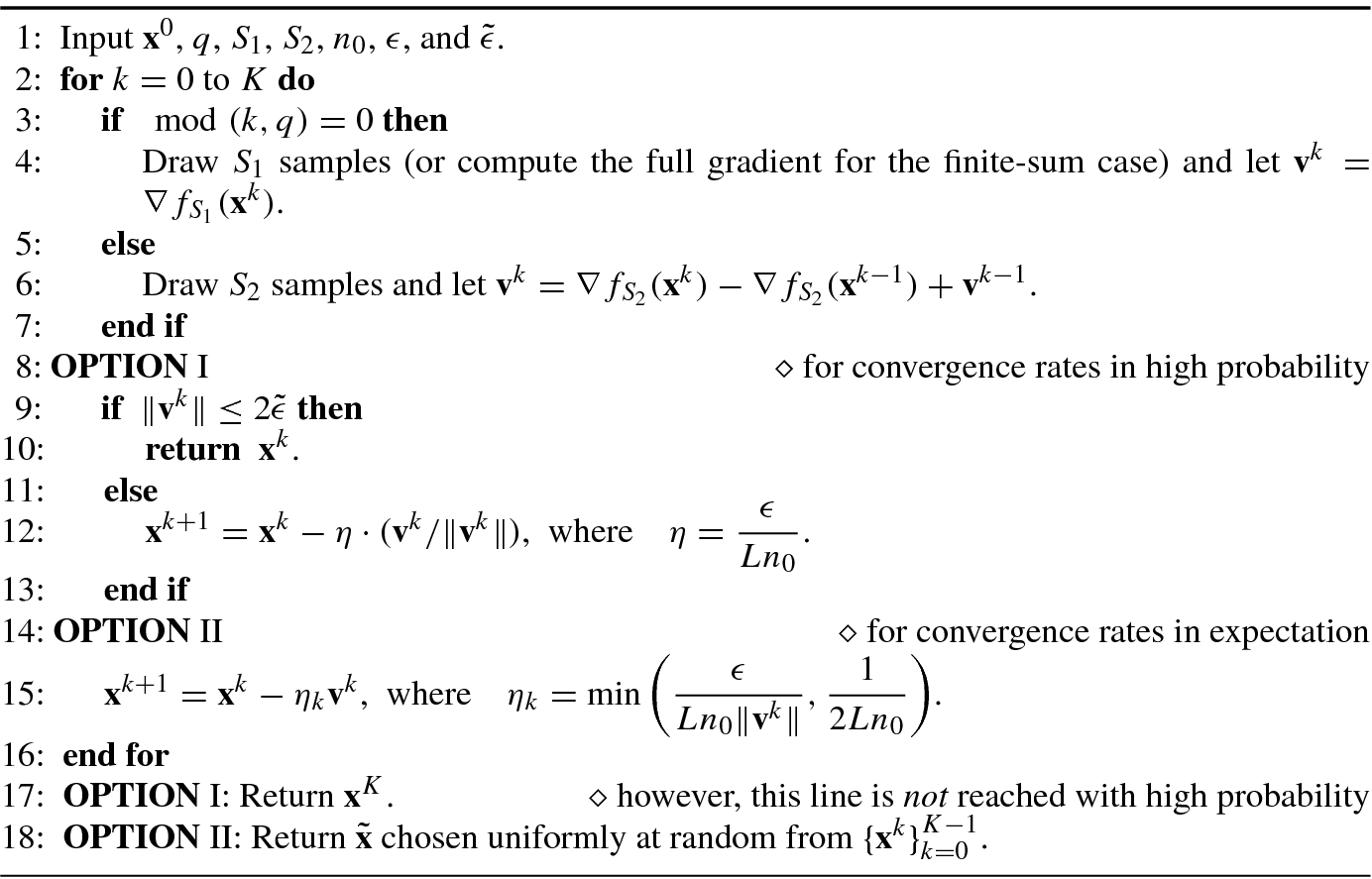
The algorithm using SPIDER to solve (5.2) is shown in Algorithm 5.5. We have the following theorem.
 . Set the parameters S
1, S
2, η, and q as
. Set the parameters S
1, S
2, η, and q as 


where Δ = f(x
0) − f
∗ (f
∗ =infxf(x)). The gradient cost is bounded by  for any choice of n
0 ∈ [1, 2σ∕𝜖]. Treating Δ, L, and σ as positive constants, the stochastic gradient complexity is O(𝜖
−3).
for any choice of n
0 ∈ [1, 2σ∕𝜖]. Treating Δ, L, and σ as positive constants, the stochastic gradient complexity is O(𝜖
−3).
To prove Theorem 5.7, we first prepare the following lemmas.
![$$\displaystyle \begin{aligned} \begin{array}{rcl}{} \mathbb{E}_{k_0} \left[\left. \left\|{\mathbf{v}}^k -\nabla f({\mathbf{x}}^k) \right \|{}^2 \right| {\mathbf{x}}_{0:k_0} \right] \leq \epsilon^2, \end{array} \end{aligned} $$](../images/487003_1_En_5_Chapter/487003_1_En_5_Chapter_TeX_Equ115.png)
where  denotes the conditional expectation over the randomness of
  .
.


![$$\displaystyle \begin{aligned} \begin{array}{rcl}{} \mathbb{E}_{k_0} \left[ f({\mathbf{x}}^{k+1}) - f({\mathbf{x}}^k) \right] \leq -\frac{\epsilon }{4Ln_0} \mathbb{E}_{k_0} \left\|{\mathbf{v}}^k\right\| + \frac{3\epsilon^2}{4n_0 L }. \end{array} \end{aligned} $$](../images/487003_1_En_5_Chapter/487003_1_En_5_Chapter_TeX_Equ119.png)


 we apply the Cauchy–Schwartz inequality. Since

 we use
  for all x. Hence
 uses
uses  .
.


Now, we are ready to prove Theorem 5.7.

 uses
uses  .
.


 in Line 17 of Algorithm 5.5, we have
 and
and  use (5.88) and (5.92), respectively.
![$$\displaystyle \begin{aligned} \begin{array}{rcl} \left\lceil K \cdot \frac{1}{q}\right\rceil S_1 + 2K S_2 &\displaystyle \overset{a}{\le}&\displaystyle 3K \cdot S_2 + S_1 \\ &\displaystyle \leq&\displaystyle \left[3\left(\frac{4Ln_0\Delta}{\epsilon^2} \right)+2\right] \frac{2\sigma}{\epsilon n_0} + \frac{2\sigma^2}{\epsilon^2}\\ &\displaystyle =&\displaystyle \frac{24L\sigma \Delta}{\epsilon^3}+ \frac{4\sigma}{n_0\epsilon} +\frac{2\sigma^2}{\epsilon^2}, \end{array} \end{aligned} $$](../images/487003_1_En_5_Chapter/487003_1_En_5_Chapter_TeX_Equ130.png)
 uses S
1 = qS
2. This concludes a gradient cost of
uses S
1 = qS
2. This concludes a gradient cost of  . □
. □
 , and let S
1 = n, i.e., we obtain the full gradient in Line 4. Then running Algorithm 5.5 with OPTION II for K iterations outputs an
, and let S
1 = n, i.e., we obtain the full gradient in Line 4. Then running Algorithm 5.5 with OPTION II for K iterations outputs an  satisfying
The gradient cost is bounded by  for any choice of n
0 ∈ [1, n
1∕2]. Treating Δ, L, and σ as positive constants, the stochastic gradient complexity is O(n + n
1∕2𝜖
−2).
for any choice of n
0 ∈ [1, n
1∕2]. Treating Δ, L, and σ as positive constants, the stochastic gradient complexity is O(n + n
1∕2𝜖
−2).

 ,
,  , and K = k − k
0 ≤ q = n
0n
1∕2, we have
, and K = k − k
0 ≤ q = n
0n
1∕2, we have 
 uses (5.96). So Lemma 5.4 holds for all k. Then from the same technique of the online case (n = ∞), we can also obtain (5.83), (5.84), and (5.93). The gradient cost analysis is computed as
 ![$$\displaystyle \begin{aligned} \begin{array}{rcl} \left\lceil K \cdot \frac{1}{q}\right\rceil S_1 + 2K S_2 &\displaystyle \overset{a}{\le}&\displaystyle 3K \cdot S_2 + S_1 \\ &\displaystyle \leq&\displaystyle \left[3\left(\frac{4Ln_0\Delta}{\epsilon^2} \right)+2\right] \frac{n^{1/2}}{n_0} + n \\ &\displaystyle =&\displaystyle \frac{12(L\Delta) \cdot n^{1/2} }{\epsilon^2}+ \frac{2n^{1/2}}{n_0} + n, \end{array} \end{aligned} $$](../images/487003_1_En_5_Chapter/487003_1_En_5_Chapter_TeX_Equ134.png)
 uses S
1 = qS
2. This concludes a gradient cost of
uses S
1 = qS
2. This concludes a gradient cost of  . □
. □5.3.2 Momentum Acceleration
When computing a first-order stationary point, SPIDER is actually (nearly) optimal, if only with the gradient-smoothness condition under certain regimes. Thus only with the condition of smoothness of the gradient, it is hard to apply the momentum techniques to accelerate algorithms. However, one can obtain a faster rate with an additional assumption on Hessian:
Each f i(x) has ρ-Lipschitz continuous Hessians (Definition A.14 ).

Suppose solving NC-Search
by [
9] and INC blocks by Catalyst
described in Theorem 5.6, the total stochastic gradient complexity to achieve an 𝜖-accuracy solution satisfying ∥∇f(x
k)∥≤ 𝜖 and  is
is  .
.
The proof of Theorem 5.9 is lengthy, so we omit the proof here. We mention that when n is large, e.g., n ≥ 𝜖
−1, the above method might not be faster than SPIDER
[7]. Thus the existing lowest complexity to find a first-order stationary point is  . In fact, for the problem of searching a stationary point in nonconvex (stochastic) optimization, neither the upper nor the lower bounds have been well studied up to now. However, it is a very hot topic recently and has aroused a lot of attention in both the optimization and the machine learning communities due to the empirical practicability for nonconvex models. Interested readers may refer to [3, 7, 9] for some latest developments.
5.4 Constrained Problem

 . We show that by fusing the VR
technique and momentum
, the convergence rate can be improved to be non-ergodic
O(1∕K).
. We show that by fusing the VR
technique and momentum
, the convergence rate can be improved to be non-ergodic
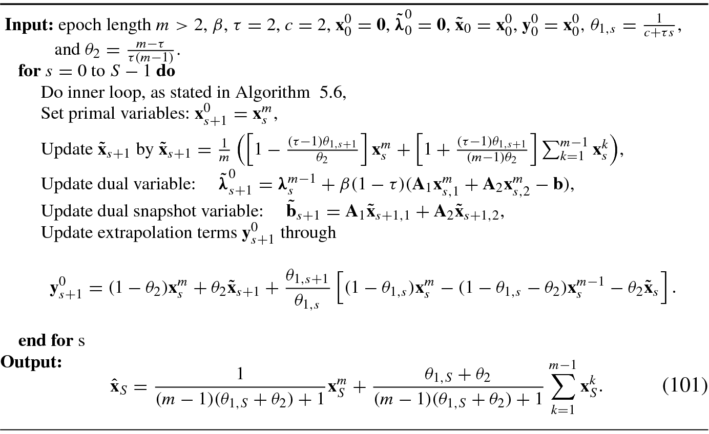
O(1∕K). and
and  through extrapolation terms
  and
and  and the dual variable
  ; in the outer loop, we maintain snapshot vectors
  ,
,  , and
, and  , and then assign the initial value to the extrapolation terms
  and
and  . The whole algorithm is shown in Algorithm 5.7. In the process of solving primal variables, we linearize both the smooth term f
i(x
i) and the augmented term
. The whole algorithm is shown in Algorithm 5.7. In the process of solving primal variables, we linearize both the smooth term f
i(x
i) and the augmented term  . The update rules of x
1 and x
2 can be written as
. The update rules of x
1 and x
2 can be written as 

 is defined as
 is a mini-batch of indices randomly chosen from [n] with a size of b.
 Notations and variables
Notation | Meaning | Variable | Meaning |
|---|---|---|---|
〈x, y〉G, ∥x∥G |
|
| Extrapolation variables |
F i(x i) | h i(x i) + f i(x i) |
| Primal variables |
x |
|
| Dual and temporary variables |
y |
|
| Snapshot vectors |
F(x) | F 1(x 1) + F 2(x 2) | used for VR | |
A | [A 1, A 2] |
| KKT point of (5.98) |
| Mini-batch indices | b | Batch size |


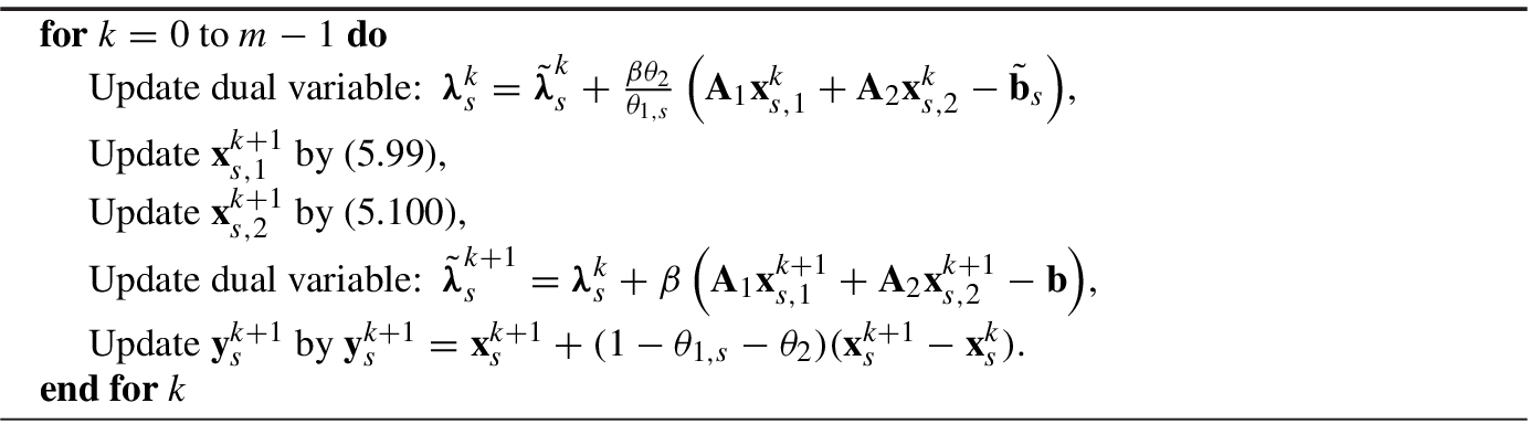
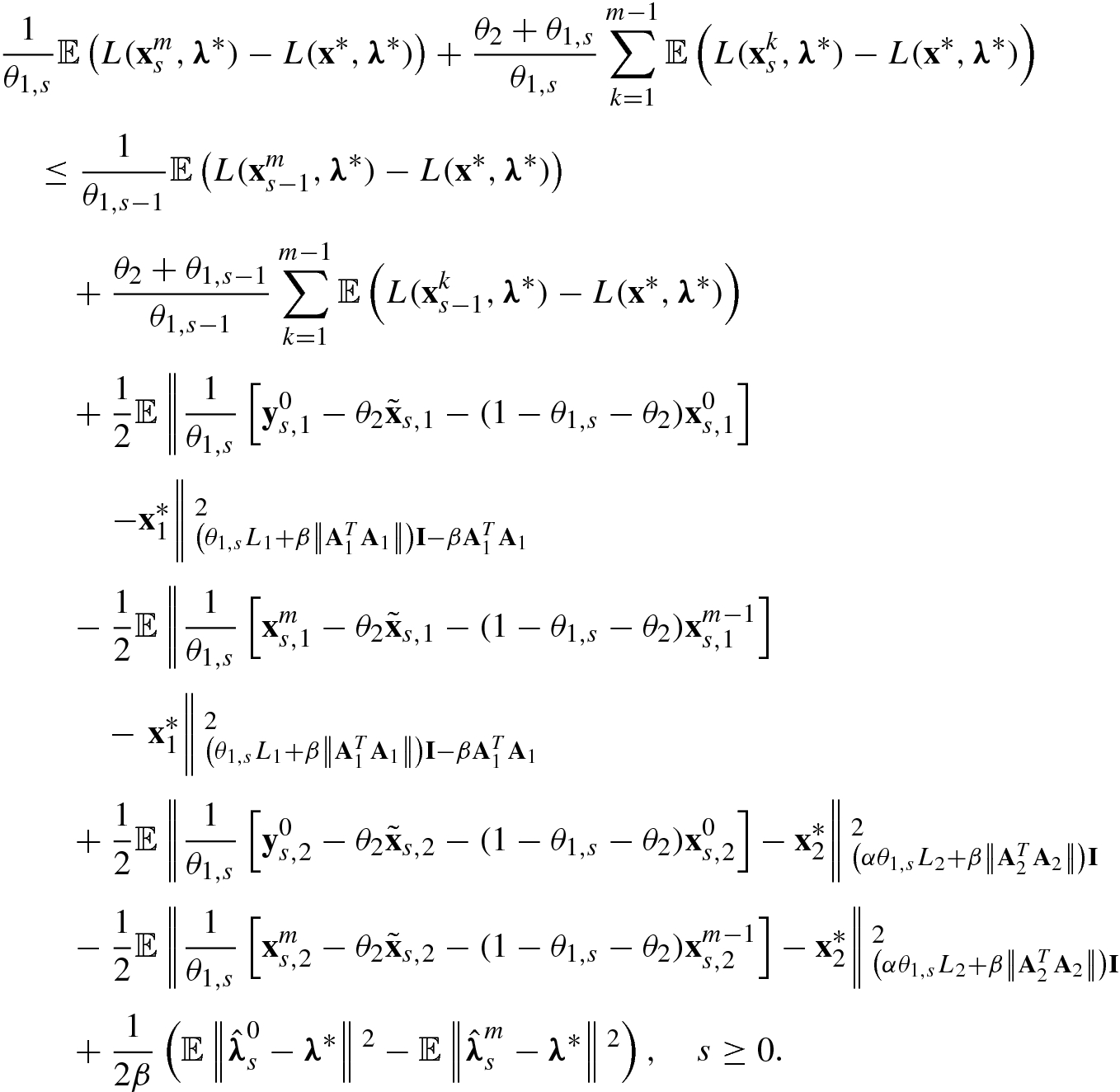
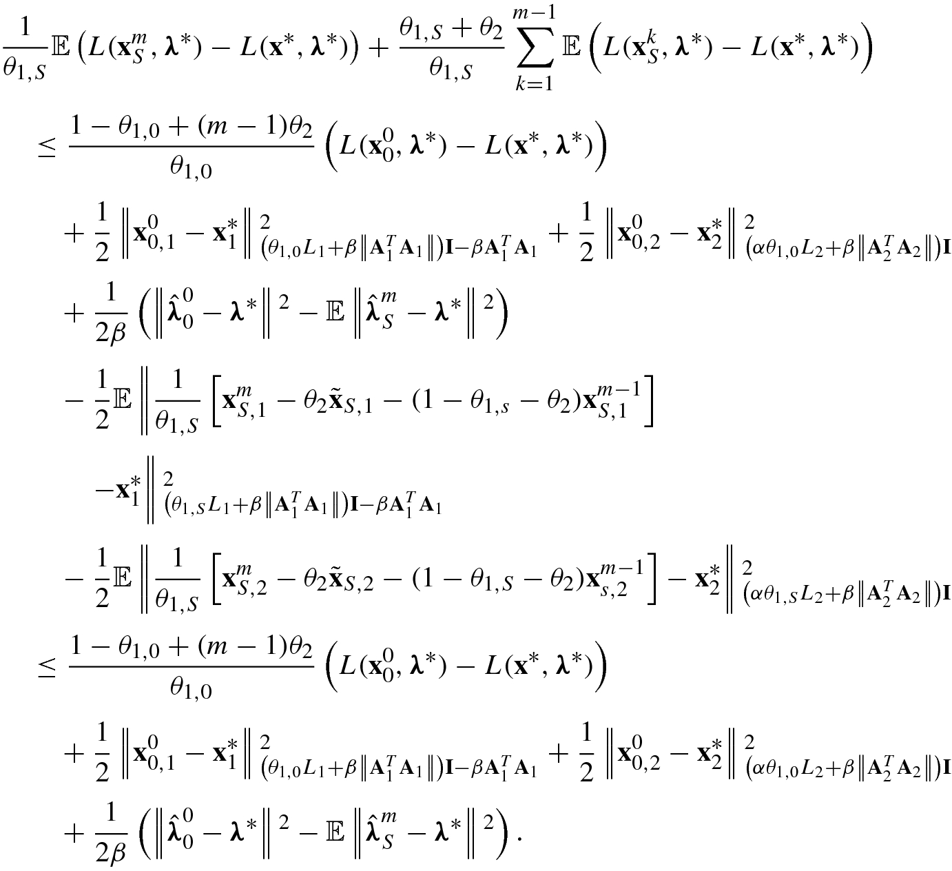
Now, we give the convergence result. The main property of Acc-SADMM (Algorithm 5.7) in the inner loop is shown below.

where  denotes that the expectation is taken over the random samples in the mini-batch
  , L(x
1, x
2, λ) = F
1(x
1) + F
2(x
2) + 〈λ, A
1x
1 + A
2x
2 −b〉 is the Lagrangian function
,
, L(x
1, x
2, λ) = F
1(x
1) + F
2(x
2) + 〈λ, A
1x
1 + A
2x
2 −b〉 is the Lagrangian function
, 
 , and
, and  . Other notations can be found in Table 5.1.
 in (5.99) and the convexity of F
1(⋅), we can obtain
in (5.99) and the convexity of F
1(⋅), we can obtain 
![$$\displaystyle \begin{aligned} \mathbb{E}_{i_k}\left\|\nabla f_2({\mathbf{y}}_2^k) - \tilde{\nabla} f_2({\mathbf{y}}_2^k)\right\|{}^2\leq \frac{2L_2}{b} \left[ f_2(\tilde{\mathbf{x}}_2) - f_2({\mathbf{y}}^k_2) - \langle \nabla f_2({\mathbf{y}}^k_2), \tilde{\mathbf{x}}_2-{\mathbf{y}}^k_2 \rangle \right]\!. \end{aligned} $$](../images/487003_1_En_5_Chapter/487003_1_En_5_Chapter_TeX_Equ141.png)

 in (5.99), we have
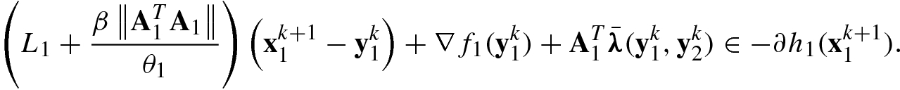

 we use the fact that f
1(⋅) is convex and so
we use the fact that f
1(⋅) is convex and so  . The inequality
  uses (5.105). Then the convexity of h
1(⋅) gives
uses (5.105). Then the convexity of h
1(⋅) gives  . So we have
 ,
,  , and
, and  , respectively, then multiplying the three inequalities by (1 − θ
1 − θ
2), θ
2, and θ
1, respectively, and adding them, we have
, respectively, then multiplying the three inequalities by (1 − θ
1 − θ
2), θ
2, and θ
1, respectively, and adding them, we have 
 we replace
  with
with  .
. in (5.100) and the convexity of F
2(⋅), we can obtain
in (5.100) and the convexity of F
2(⋅), we can obtain 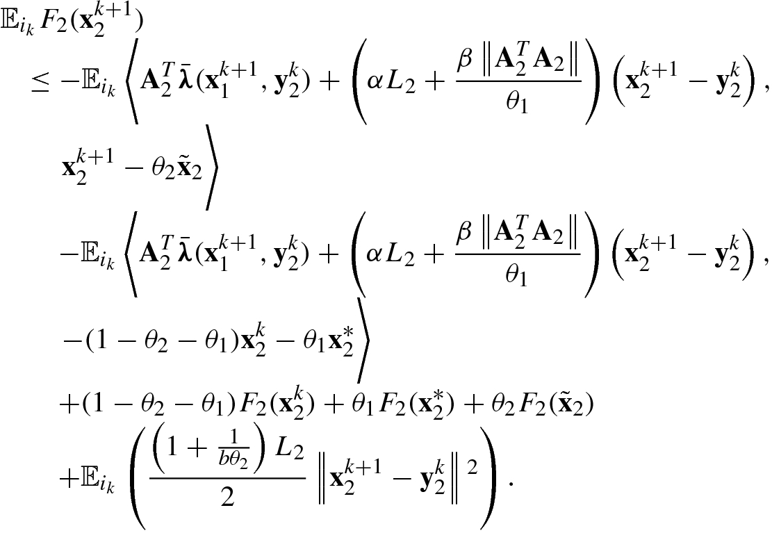
 in (5.100), we have
 . Since f
2 is L
2-smooth, we have
. Since f
2 is L
2-smooth, we have 
 and have
 we introduce an arbitrary variable u
2 (we will set it to be
we introduce an arbitrary variable u
2 (we will set it to be  ,
,  , and
, and  ) and in the equality
  we set
 , we have
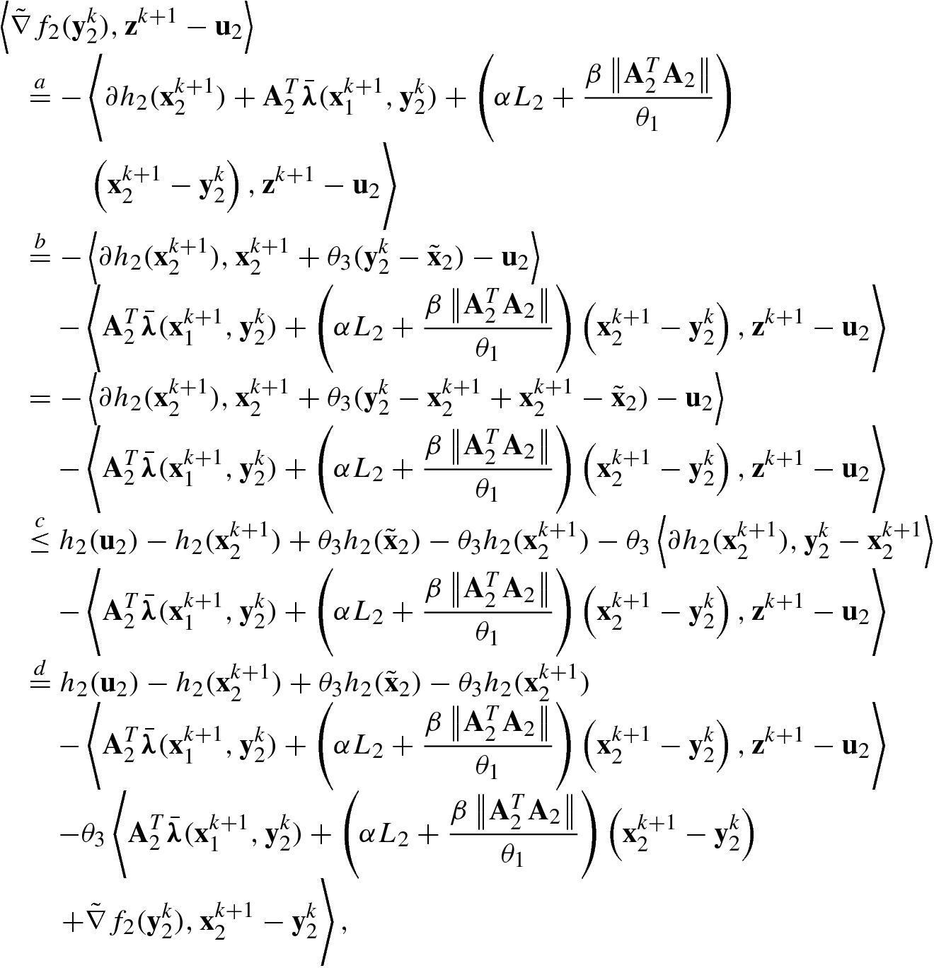
 and
and  , we use (5.108) and (5.111), respectively. The inequality
  uses (5.108) again. The inequality
  uses the convexity of h
2:
uses the convexity of h
2: 
 , we have
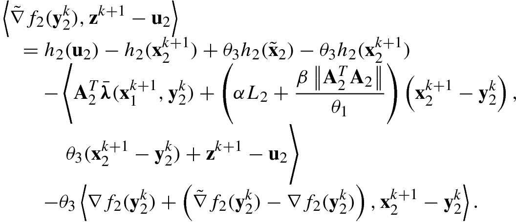

 and obtain
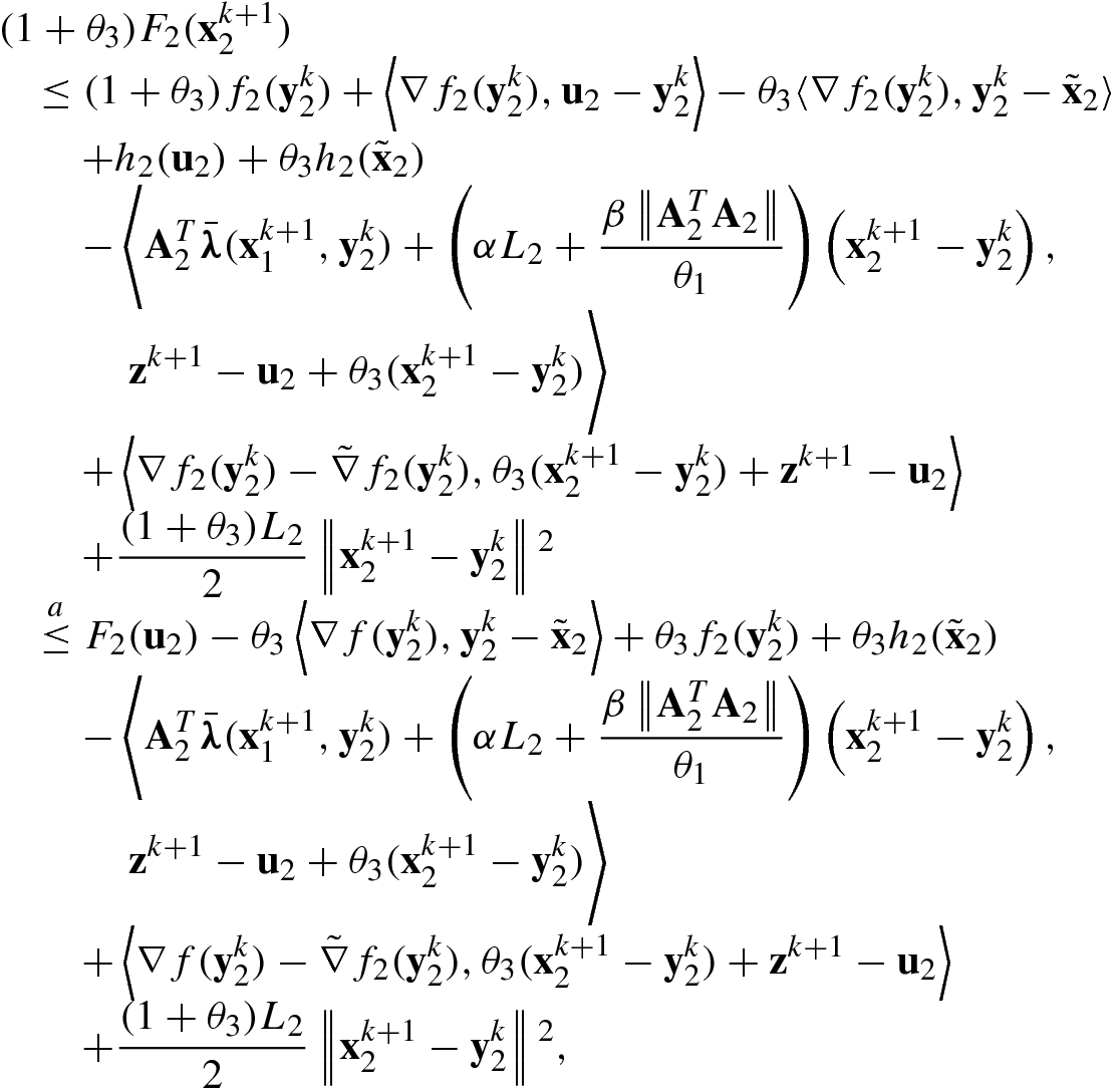
 uses the convexity of f
2:
uses the convexity of f
2: 
 . We will set u
2 to be
. We will set u
2 to be  and
and  , which do not depend on
  . So we obtain
 we use the fact that
 ,
,  ,
,  , and u
2 are independent of i
k,s (they are known), so
, and u
2 are independent of i
k,s (they are known), so 
 and
and  hold similarly; the inequality
  uses the Cauchy–Schwartz inequality; and
  uses (5.104). Taking expectation on (5.115) and adding (5.116), we obtain
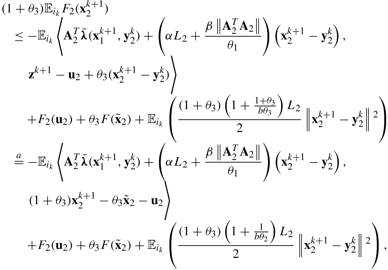
 we use (5.111) and set θ
3 satisfying
we use (5.111) and set θ
3 satisfying  . Setting u
2 to be
. Setting u
2 to be  and
and  , respectively, then multiplying the two inequalities by 1 − θ
1(1 + θ
3) and θ
1(1 + θ
3), respectively, and adding them, we obtain
, respectively, then multiplying the two inequalities by 1 − θ
1(1 + θ
3) and θ
1(1 + θ
3), respectively, and adding them, we obtain 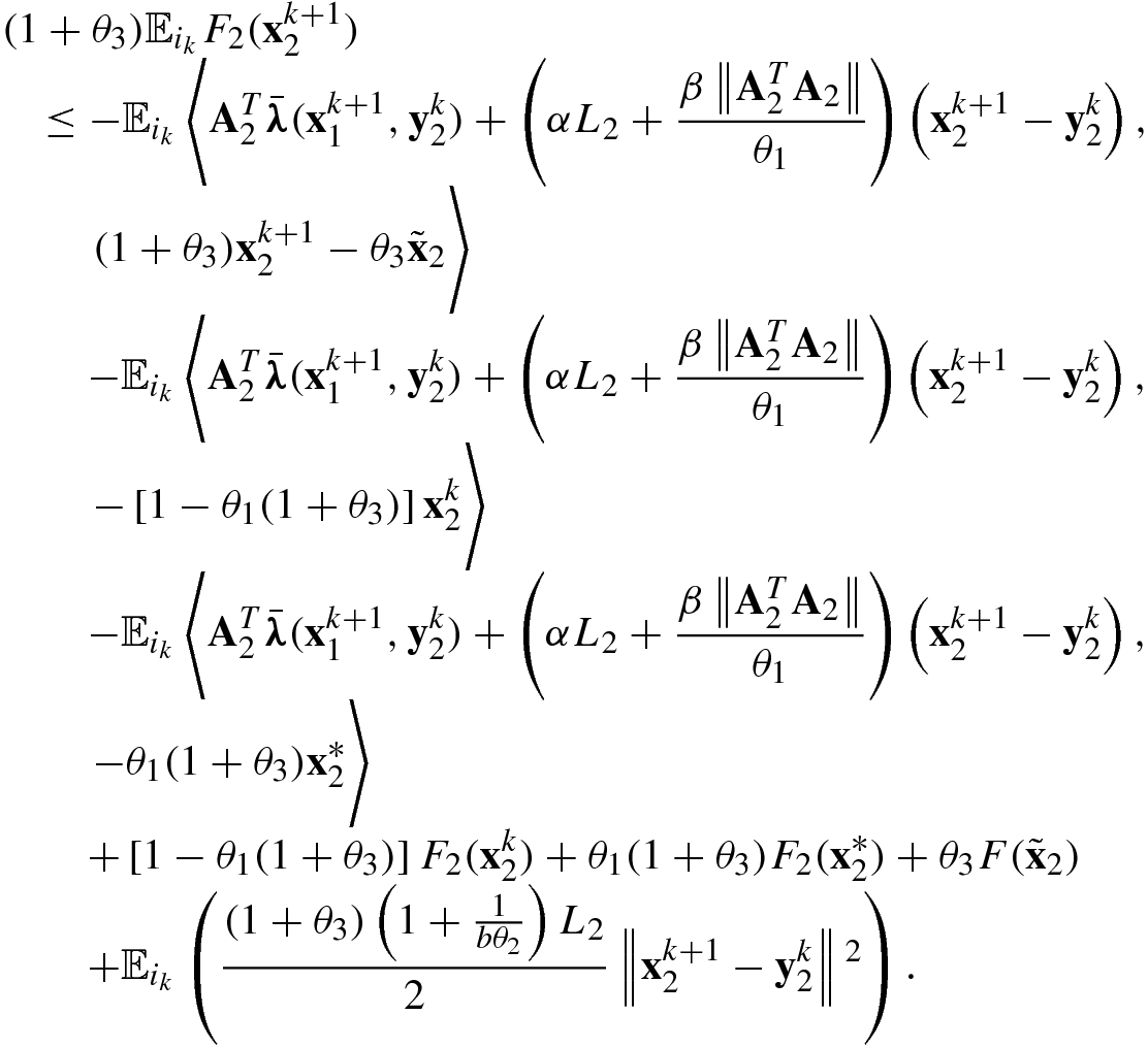
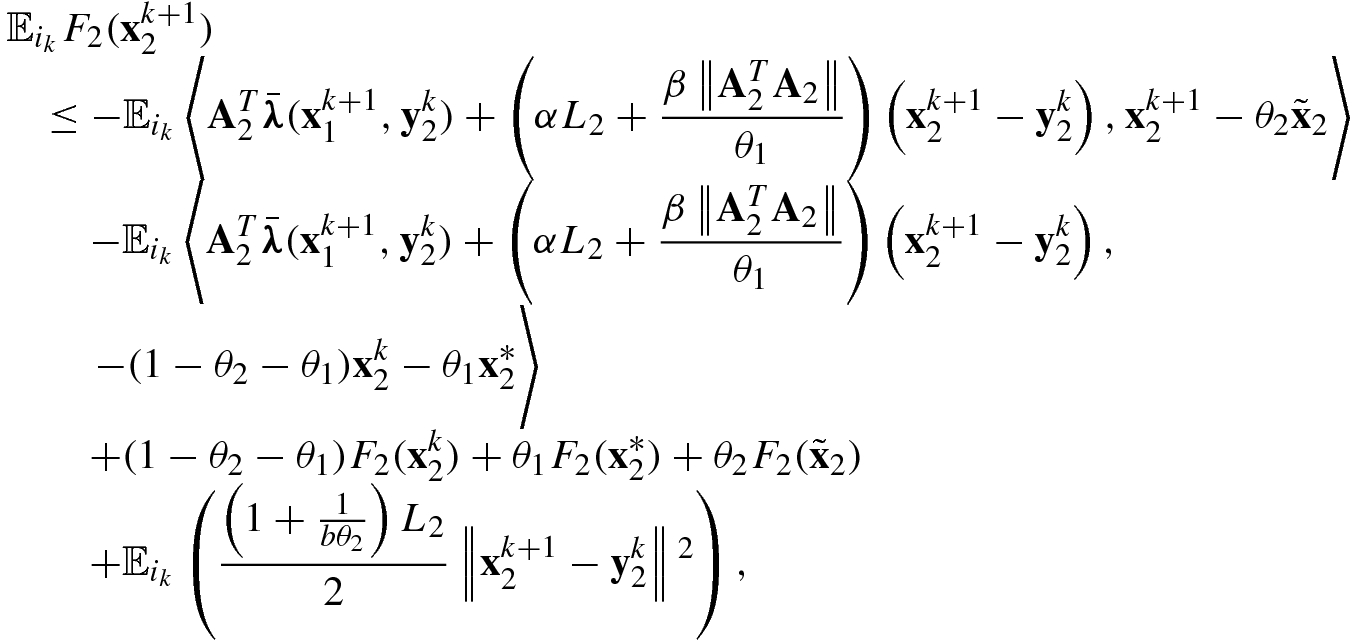
 and so
  . We obtain (5.107).

![$$\displaystyle \begin{aligned} \begin{array}{rcl} \hat{\boldsymbol\lambda}^{k+1}-\hat{\boldsymbol\lambda}^{k}&\displaystyle =&\displaystyle \frac{\beta }{\theta_1}{\mathbf{A}}_1\left[{\mathbf{x}}^{k+1}_1-(1-\theta_1-\theta_2){\mathbf{x}}_1^{k} -\theta_2\tilde{\mathbf{x}}_1-\theta_1{\mathbf{x}}_1^*\right]\\ &\displaystyle &\displaystyle + \frac{\beta }{\theta_1}{\mathbf{A}}_2\left[{\mathbf{x}}^{k+1}_2-(1-\theta_1-\theta_2){\mathbf{x}}_2^{k} -\theta_2\tilde{\mathbf{x}}_2-\theta_1{\mathbf{x}}_2^* \right],{} \end{array} \end{aligned} $$](../images/487003_1_En_5_Chapter/487003_1_En_5_Chapter_TeX_Equ161.png)


![$$\displaystyle \begin{aligned} \begin{array}{rcl} \hat{\boldsymbol\lambda}^{k+1} &\displaystyle =&\displaystyle \tilde{\boldsymbol\lambda}^{k+1} +\beta \left(\frac{1}{\theta_1}-1\right)({\mathbf{A}}_1{\mathbf{x}}^{k+1}_1+{\mathbf{A}}_2{\mathbf{x}}^{k+1}_2-{\mathbf{b}})\\ &\displaystyle \overset{a}=&\displaystyle \boldsymbol\lambda^{k} +\frac{\beta }{\theta_1}({\mathbf{A}}_1{\mathbf{x}}^{k+1}_1+{\mathbf{A}}_2{\mathbf{x}}^{k+1}_2-{\mathbf{b}}){}\\ &\displaystyle \overset{b}=&\displaystyle \tilde{\boldsymbol\lambda}^k +\frac{\beta}{\theta_1}\left\{ {\mathbf{A}}_1{\mathbf{x}}^{k+1}_1+{\mathbf{A}}_2{\mathbf{x}}^{k+1}_2-{\mathbf{b}} +\theta_2\left[ {\mathbf{A}}_1({\mathbf{x}}^{k}_2-\tilde{\mathbf{x}}_1) + {\mathbf{A}}_2({\mathbf{x}}^{k}_2-\tilde{\mathbf{x}}_2)\right] \right\}, \end{array} \end{aligned} $$](../images/487003_1_En_5_Chapter/487003_1_En_5_Chapter_TeX_Equ165.png)
 we use (5.124) and the equality
  is obtained by (5.123) and
  (see Algorithm 5.7). Together with (5.119) we obtain
 ![$$\displaystyle \begin{aligned} \begin{array}{rcl} \hat{\boldsymbol\lambda}^{k+1}-\hat{\boldsymbol\lambda}^{k} &\displaystyle =&\displaystyle \frac{\beta }{\theta_1}{\mathbf{A}}_1\left[{\mathbf{x}}^{k+1}_1-(1-\theta_1){\mathbf{x}}_1^{k}-\theta_1{\mathbf{x}}_1^* +\theta_2({\mathbf{x}}^k_1-\tilde{\mathbf{x}}_1)\right]\\ &\displaystyle &\displaystyle + \frac{\beta }{\theta_1}{\mathbf{A}}_2\left[{\mathbf{x}}^{k+1}_2-(1-\theta_1){\mathbf{x}}_2^{k}-\theta_1{\mathbf{x}}_2^* +\theta_2({\mathbf{x}}^k_2-\tilde{\mathbf{x}}_2) \right], \end{array} \end{aligned} $$](../images/487003_1_En_5_Chapter/487003_1_En_5_Chapter_TeX_Equ166.png)
 . So (5.121) is proven.
 , we obtain (5.120). Now we prove
  when s ≥ 1.
 uses (5.119),
  uses the fact that
  ,
,  uses
uses  in Algorithm 5.7, and
  uses (5.124).
 . We have
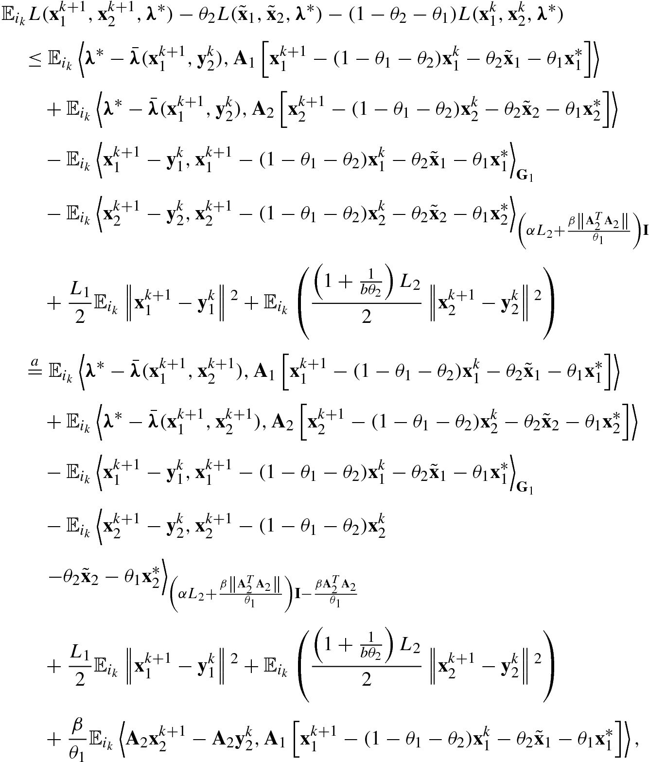
 ![$$\displaystyle \begin{aligned} \begin{array}{rcl} &\displaystyle &\displaystyle L({\mathbf{x}}^{k+1}_1,{\mathbf{x}}^{k+1}_2,\boldsymbol\lambda^*) - \theta_2 L(\tilde{\mathbf{x}}_1,\tilde{\mathbf{x}}_2,\boldsymbol\lambda^*) -(1-\theta_1 - \theta_2)L({\mathbf{x}}^{k}_1,{\mathbf{x}}^{k}_2,\boldsymbol\lambda^*)\\ &\displaystyle &\displaystyle \quad = F_1({\mathbf{x}}^{k+1}_1)-(1-\theta_2-\theta_1)F_1({\mathbf{x}}^{k}_1) -\theta_1F_1({\mathbf{x}}^*_1) -\theta_2 F_1(\tilde{\mathbf{x}}_1)\\ &\displaystyle &\displaystyle \qquad +F_2({\mathbf{x}}^{k+1}_2)-(1-\theta_2-\theta_1)F_2({\mathbf{x}}^{k}_2) -\theta_1F_2({\mathbf{x}}^*_2) -\theta_2 F_2(\tilde{\mathbf{x}}_2)\\ &\displaystyle &\displaystyle \qquad + \left\langle \boldsymbol\lambda^*, {\mathbf{A}}_1\left[{\mathbf{x}}^{k+1}_1-(1-\theta_1-\theta_2){\mathbf{x}}_1^{k}-\theta_2\tilde{\mathbf{x}}_1-\theta_1 {\mathbf{x}}_1^*\right] \right\rangle\\ &\displaystyle &\displaystyle \qquad + \left\langle \boldsymbol\lambda^*, {\mathbf{A}}_2\left[{\mathbf{x}}^{k+1}_2-(1-\theta_1-\theta_2){\mathbf{x}}_2^{k}-\theta_2\tilde{\mathbf{x}}_2-\theta_1 {\mathbf{x}}_2^*\right] \right\rangle. \end{array} \end{aligned} $$](../images/487003_1_En_5_Chapter/487003_1_En_5_Chapter_TeX_Equ168.png)
 we change the term
  to
to  . For the first two terms in the right-hand side of (5.127), we have
 ![$$\displaystyle \begin{aligned} \begin{array}{rcl}{} &\displaystyle &\displaystyle \left\langle \boldsymbol\lambda^*-{\bar{\boldsymbol\lambda}}({\mathbf{x}}^{k+1}_1,{\mathbf{x}}^{k+1}_2), {\mathbf{A}}_1\left[{\mathbf{x}}^{k+1}_1-(1-\theta_1-\theta_2){\mathbf{x}}_1^{k}-\theta_2\tilde{\mathbf{x}}_1-\theta_1{\mathbf{x}}_1^*\right] \right\rangle\\ &\displaystyle &\displaystyle \quad +\left\langle \boldsymbol\lambda^*-{\bar{\boldsymbol\lambda}}({\mathbf{x}}^{k+1}_1,{\mathbf{x}}^{k+1}_2), {\mathbf{A}}_2\left[{\mathbf{x}}^{k+1}_2-(1-\theta_1-\theta_2){\mathbf{x}}_1^{k}-\theta_2\tilde{\mathbf{x}}_2-\theta_1 {\mathbf{x}}_2^*\right] \right\rangle\\ &\displaystyle &\displaystyle \qquad \overset{a}= \frac{\theta_1}{\beta} \langle \boldsymbol\lambda^*-\hat{\boldsymbol\lambda}^{k+1}, \hat{\boldsymbol\lambda}^{k+1}-\hat{\boldsymbol\lambda}^{k}\rangle\\ &\displaystyle &\displaystyle \qquad \overset{b}= \frac{\theta_1}{2\beta}\left(\left\|\hat{\boldsymbol\lambda}^k-\boldsymbol\lambda^*\right\|{}^2- \left\|\hat{\boldsymbol\lambda}^{k+1}-\boldsymbol\lambda^*\right\|{}^2 -\left\| \hat{\boldsymbol\lambda}^{k+1} -\hat{\boldsymbol\lambda}^{k}\right\|{}^2\right), \end{array} \end{aligned} $$](../images/487003_1_En_5_Chapter/487003_1_En_5_Chapter_TeX_Equ170.png)
 uses (5.120) and (5.121) and
  uses (A.2).
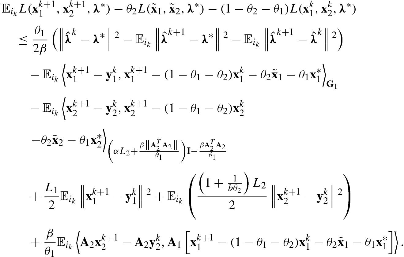
![$$\displaystyle \begin{aligned} & \mathbb{E}_{i_k}L({\mathbf{x}}^{k+1}_1,{\mathbf{x}}^{k+1}_2,\boldsymbol\lambda^*) - \theta_2 L(\tilde{\mathbf{x}}_1,\tilde{\mathbf{x}}_2,\boldsymbol\lambda^*) -(1-\theta_2 - \theta_1)L({\mathbf{x}}^{k}_1,{\mathbf{x}}^{k}_2,\boldsymbol\lambda^*)\\ &\quad \leq \frac{\theta_1}{2\beta}\left(\left\|\hat{\boldsymbol\lambda}^k-\boldsymbol\lambda^*\right\|{}^2- \mathbb{E}_{i_k}\left\|\hat{\boldsymbol\lambda}^{k+1}-\boldsymbol\lambda^*\right\|{}^2 -\mathbb{E}_{i_k}\left\| \hat{\boldsymbol\lambda}^{k+1} -\hat{\boldsymbol\lambda}^{k}\right\|{}^2\right)\\ &\qquad +\frac{1}{2}\left\|{\mathbf{y}}_1^{k}-(1-\theta_1-\theta_2){\mathbf{x}}_1^{k}-\theta_2\tilde{\mathbf{x}}_1-\theta_1{\mathbf{x}}_1^*\right\|{}^2_{{\mathbf{G}}_1}\\ &\qquad -\frac{1}{2}\mathbb{E}_{i_k}\left\|{\mathbf{x}}^{k+1}_1-(1-\theta_1-\theta_2){\mathbf{x}}_1^{k}-\theta_2\tilde{\mathbf{x}}_1-\theta_1{\mathbf{x}}_1^*\right\|{}^2_{{\mathbf{G}}_1}\\ &\qquad + \frac{1}{2} \left\|{\mathbf{y}}_2^{k}-(1-\theta_1-\theta_2){\mathbf{x}}^k_2-\theta_2\tilde{\mathbf{x}}_2-\theta_1{\mathbf{x}}_2^*\right\|{}^2_{\left(\alpha L_2+\frac{\beta\left\|{\mathbf{A}}_2^T {\mathbf{A}}_2\right\|}{\theta_1}\right)\mathbf{I}-\frac{\beta{\mathbf{A}}_2^T{\mathbf{A}}_2}{\theta_1}}\\ &\qquad -\frac{1}{2} \mathbb{E}_{i_k} \left\|{\mathbf{x}}_2^{k+1}-(1-\theta_1-\theta_2){\mathbf{x}}^k_2-\theta_2\tilde{\mathbf{x}}_2-\theta_1{\mathbf{x}}_2^*\right\|{}^2_{\left(\alpha L_2+\frac{\beta\left\|{\mathbf{A}}_2^T {\mathbf{A}}_2\right\|}{\theta_1}\right)\mathbf{I}-\frac{\beta{\mathbf{A}}_2^T{\mathbf{A}}_2}{\theta_1}}\\ &\qquad -\frac{1}{2}\mathbb{E}_{i_k}\left\|{\mathbf{x}}^{k+1}_1-{\mathbf{y}}^k_1 \right \|{}^2_{\frac{\beta\left\|{\mathbf{A}}_1^T {\mathbf{A}}_1\right\|}{\theta_1}\mathbf{I}-\frac{\beta{\mathbf{A}}_1^T{\mathbf{A}}_1}{\theta_1} }-\frac{1}{2}\mathbb{E}_{i_k}\left\|{\mathbf{x}}^{k+1}_2-{\mathbf{y}}^k_2\right\|{}^2_{\frac{\beta\left\|{\mathbf{A}}_2^T {\mathbf{A}}_2\right\|}{\theta_1}\mathbf{I}-\frac{\beta{\mathbf{A}}_2^T{\mathbf{A}}_2}{\theta_1} } \\ &\qquad +\frac{\beta}{\theta_1}\mathbb{E}_{i_k}\left\langle {\mathbf{A}}_2{\mathbf{x}}^{k+1}_2-{\mathbf{A}}_2{\mathbf{y}}^{k}_2,{\mathbf{A}}_1\left[{\mathbf{x}}^{k+1}_1-(1-\theta_1-\theta_2){\mathbf{x}}_1^{k}-\theta_2\tilde{\mathbf{x}}_1-\theta_1 {\mathbf{x}}_1^*\right] \right\rangle\!. \end{aligned} $$](../images/487003_1_En_5_Chapter/487003_1_En_5_Chapter_TeX_Equ172.png)
![$$\displaystyle \begin{aligned} &\frac{\beta}{\theta_1}\left\langle {\mathbf{A}}_2{\mathbf{x}}^{k+1}_2-{\mathbf{A}}_2{\mathbf{y}}^{k}_2,{\mathbf{A}}_1\left[{\mathbf{x}}^{k+1}_1-(1-\theta_1-\theta_2){\mathbf{x}}_1^{k}-\theta_2\tilde{\mathbf{x}}_1-\theta_1{\mathbf{x}}_1^*\right] \right\rangle\\ &\quad \overset{a}=\frac{\beta}{\theta_1}\left\langle {\mathbf{A}}_2{\mathbf{x}}^{k+1}_2\!\!-\!{\mathbf{A}}_2\mathbf{v} -({\mathbf{A}}_2{\mathbf{y}}^{k}_2-{\mathbf{A}}_2\mathbf{v}),\right. \\ &\qquad \left.{\mathbf{A}}_1\!\!\left[{\mathbf{x}}^{k+1}_1\!\!-(1\!-\!\theta_1-\!\theta_2){\mathbf{x}}_1^{k}-\theta_2\tilde{\mathbf{x}}_1-\theta_1{\mathbf{x}}_1^*\right] \!\!-\!\mathbf{0} \right\rangle\\ &\quad \overset{b}=\frac{\beta}{2\theta_1}\left\|{\mathbf{A}}_2{\mathbf{x}}^{k+1}_2 -{\mathbf{A}}_2 \mathbf{v}+ {\mathbf{A}}_1\left[{\mathbf{x}}^{k+1}_1-(1-\theta_1-\theta_2){\mathbf{x}}_1^{k}-\theta_2\tilde{\mathbf{x}}_1-\theta_1{\mathbf{x}}_1^*\right] \right\|{}^2\\ &\qquad -\frac{\beta}{2\theta_1}\left\|{\mathbf{A}}_2{\mathbf{x}}^{k+1}_2-{\mathbf{A}}_2\mathbf{v} \right\|{}^2+\frac{\beta}{2\theta_1}\left\|{\mathbf{A}}_2{\mathbf{y}}^{k}_2-{\mathbf{A}}_2\mathbf{v} \right\|{}^2\\ &\qquad -\frac{\beta}{2\theta_1}\left\|{\mathbf{A}}_2{\mathbf{y}}^{k}_2-{\mathbf{A}}_2 \mathbf{v} + {\mathbf{A}}_1\left[{\mathbf{x}}^{k+1}_1-(1-\theta_1-\theta_2){\mathbf{x}}_1^{k}-\theta_2\tilde{\mathbf{x}}_1-\theta_1{\mathbf{x}}_1^*\right] \right\|{}^2\\ &\quad \overset{c}= \frac{\theta_1}{2\beta}\left\| \hat{\boldsymbol\lambda}^{k+1} -\hat{\boldsymbol\lambda}^{k} \right\|{}^2 -\frac{\beta}{2\theta_1}\left\|{\mathbf{A}}_2{\mathbf{x}}^{k+1}_2-{\mathbf{A}}_2\mathbf{v} \right\|{}^2+\frac{\beta}{2\theta_1}\left\|{\mathbf{A}}_2{\mathbf{y}}^{k}_2-{\mathbf{A}}_2\mathbf{v} \right\|{}^2\\ &\qquad -\frac{\beta}{2\theta_1}\left\|{\mathbf{A}}_2{\mathbf{y}}^{k}_2-{\mathbf{A}}_2 \mathbf{v} + {\mathbf{A}}_1\left[{\mathbf{x}}^{k+1}_1-(1-\theta_1-\theta_2){\mathbf{x}}_1^{k}-\theta_2\tilde{\mathbf{x}}_1-\theta_1{\mathbf{x}}_1^*\right] \right \|{}^2,\end{aligned} $$](../images/487003_1_En_5_Chapter/487003_1_En_5_Chapter_TeX_Equ173.png)


![$$\displaystyle \begin{aligned} \begin{array}{rcl}{} &\displaystyle &\displaystyle \mathbb{E}_{i_k}L({\mathbf{x}}^{k+1}_1,{\mathbf{x}}^{k+1}_2,\boldsymbol\lambda^*) - \theta_2 L(\tilde{\mathbf{x}}_1,\tilde{\mathbf{x}}_2,\boldsymbol\lambda^*) -(1-\theta_2 - \theta_1)L({\mathbf{x}}^{k}_1,{\mathbf{x}}^{k}_2,\boldsymbol\lambda^*)\\ &\displaystyle &\displaystyle \quad \leq \frac{\theta_1}{2\beta}\left( \left\|\hat{\boldsymbol\lambda}^k-\boldsymbol\lambda^*\right\|{}^2- \mathbb{E}_{i_k}\left\|\hat{\boldsymbol\lambda}^{k+1}-\boldsymbol\lambda^*\right\|{}^2 \right)\\ &\displaystyle &\displaystyle \qquad +\frac{1}{2}\left\|{\mathbf{y}}_1^{k}-(1-\theta_1-\theta_2){\mathbf{x}}_1^{k}-\theta_2\tilde{\mathbf{x}}_1-\theta_1{\mathbf{x}}_1^*\right\|{}^2_{{\mathbf{G}}_1}\\ &\displaystyle &\displaystyle \qquad -\frac{1}{2}\mathbb{E}_{i_k}\left\|{\mathbf{x}}^{k+1}_1-(1-\theta_1-\theta_2){\mathbf{x}}_1^{k}-\theta_2\tilde{\mathbf{x}}_1-\theta_1{\mathbf{x}}_1^*\right\|{}^2_{{\mathbf{G}}_1}\\ &\displaystyle &\displaystyle \qquad + \frac{1}{2} \left\|{\mathbf{y}}_2^{k}-(1-\theta_1-\theta_2){\mathbf{x}}^k_2-\theta_2\tilde{\mathbf{x}}_2-\theta_1{\mathbf{x}}_2^*\right\|{}^2_{\left(\alpha L_2+\frac{\beta\left\|{\mathbf{A}}_2^T {\mathbf{A}}_2\right\|}{\theta_1}\right)\mathbf{I}}\\ &\displaystyle &\displaystyle \qquad - \frac{1}{2}\mathbb{E}_{i_k}\left\|{\mathbf{x}}_2^{k+1} - (1-\theta_1 - \theta_2){\mathbf{x}}^k_2-\theta_2 \tilde{\mathbf{x}}_2 - \theta_1 {\mathbf{x}}^*_2 \right\|{}^2_{\left(\alpha L_2+\frac{\beta\left\|{\mathbf{A}}_2^T {\mathbf{A}}_2\right\|}{\theta_1}\right)\mathbf{I}}\\ &\displaystyle &\displaystyle \qquad -\frac{1}{2}\mathbb{E}_{i_k}\left\|{\mathbf{x}}^{k+1}_1-{\mathbf{y}}^k_1 \right\|{}^2_{\frac{\beta\left\|{\mathbf{A}}_1^T {\mathbf{A}}_1\right\|}{\theta_1}\mathbf{I}-\frac{\beta{\mathbf{A}}_1^T{\mathbf{A}}_1}{\theta_1} }-\frac{1}{2}\mathbb{E}_{i_k}\left\|{\mathbf{x}}^{k+1}_2-{\mathbf{y}}^k_2\right\|{}^2_{\frac{\beta\left\|{\mathbf{A}}_2^T {\mathbf{A}}_2\right\|}{\theta_1}\mathbf{I}-\frac{\beta{\mathbf{A}}_2^T{\mathbf{A}}_2}{\theta_1} } \\ &\displaystyle &\displaystyle \qquad -\frac{\beta}{2\theta_1}\mathbb{E}_{i_k}\left\|{\mathbf{A}}_2{\mathbf{y}}^{k}_2-{\mathbf{A}}_2 \mathbf{v} + {\mathbf{A}}_1\left[{\mathbf{x}}^{k+1}_1-(1-\theta_1-\theta_2){\mathbf{x}}_1^{k}-\theta_2\tilde{\mathbf{x}}_1-\theta_1{\mathbf{x}}_1^*\right] \right \|{}^2.\\ \end{array} \end{aligned} $$](../images/487003_1_En_5_Chapter/487003_1_En_5_Chapter_TeX_Equ174.png)


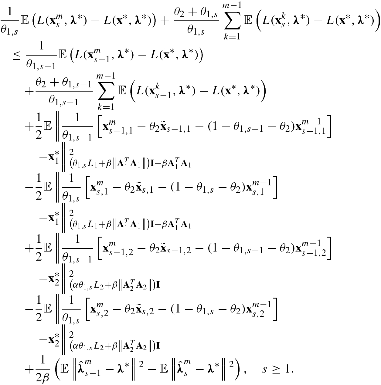
![$$\displaystyle \begin{aligned} &\frac{1}{\theta_{1}}\mathbb{E} L({\mathbf{x}}^{k+1}_1,{\mathbf{x}}^{k+1}_2,\boldsymbol\lambda^*) - \frac{\theta_2}{\theta_{1}} L(\tilde{\mathbf{x}}_1,\tilde{\mathbf{x}}_2,\boldsymbol\lambda^*) -\frac{1-\theta_2 - \theta_1}{\theta_{1}}L({\mathbf{x}}^{k}_1,{\mathbf{x}}^{k}_2,\boldsymbol\lambda^*)\\ &\quad \leq \frac{1}{2\beta}\left(\left\|\hat{\boldsymbol\lambda}^k-\boldsymbol\lambda^*\right\|{}^2- \mathbb{E}\left\|\hat{\boldsymbol\lambda}^{k+1}-\boldsymbol\lambda^*\right\|{}^2 \right) \\ &\qquad +\frac{\theta_{1}}{2}\left\|\frac{1}{\theta_1}\left[{\mathbf{y}}_1^{k}-(1-\theta_1-\theta_2){\mathbf{x}}_1^{k}-\theta_2\tilde{\mathbf{x}}_1\right]-{\mathbf{x}}_1^*\right\|{}^2_{\left(L_1+\frac{\beta\left\|{\mathbf{A}}_1^T {\mathbf{A}}_1\right\|}{\theta_1}\right)\mathbf{I}-\frac{\beta{\mathbf{A}}_1^T{\mathbf{A}}_1}{\theta_1} }\\ &\qquad -\frac{\theta_{1}}{2}\mathbb{E}\left\|\frac{1}{\theta_1}\left[{\mathbf{x}}^{k+1}_1-(1-\theta_1-\theta_2){\mathbf{x}}_1^{k}-\theta_2\tilde{\mathbf{x}}_1\right]-{\mathbf{x}}_1^*\right\|{}^2_{\left(L_1+\frac{\beta\left\|{\mathbf{A}}_1^T {\mathbf{A}}_1\right\|}{\theta_1}\right)\mathbf{I}-\frac{\beta{\mathbf{A}}_1^T{\mathbf{A}}_1}{\theta_1} }\\ &\qquad + \frac{\theta_{1}}{2} \left\|\frac{1}{\theta_1}\left[{\mathbf{y}}_2^{k}-(1-\theta_1-\theta_2){\mathbf{x}}^k_2-\theta_2\tilde{\mathbf{x}}_2\right]-{\mathbf{x}}_2^*\right\|{}^2_{\left(\alpha L_2+\frac{\beta\left\|{\mathbf{A}}_2^T {\mathbf{A}}_2\right\|}{\theta_1}\right)\mathbf{I}}\\ &\qquad -\frac{\theta_{1}}{2} \mathbb{E} \left\|\frac{1}{\theta_1}\left[{\mathbf{x}}_2^{k+1}-(1-\theta_1-\theta_2){\mathbf{x}}^k_2-\theta_2\tilde{\mathbf{x}}_2\right]-{\mathbf{x}}_2^*\right\|{}^2_{\left(\alpha L_2+\frac{\beta\left\|{\mathbf{A}}_2^T {\mathbf{A}}_2\right\|}{\theta_1}\right)\mathbf{I}}, \end{aligned} $$](../images/487003_1_En_5_Chapter/487003_1_En_5_Chapter_TeX_Equ176.png)

![$$\displaystyle \begin{aligned} &\frac{1}{\theta_{1}}\mathbb{E} L({\mathbf{x}}^{k+1}_1,{\mathbf{x}}^{k+1}_2,\boldsymbol\lambda^*) - \frac{\theta_2}{\theta_{1}} L(\tilde{\mathbf{x}}_1,\tilde{\mathbf{x}}_2,\boldsymbol\lambda^*) -\frac{1-\theta_2 - \theta_1}{\theta_{1}}L({\mathbf{x}}^{k}_1,{\mathbf{x}}^{k}_2,\boldsymbol\lambda^*)\\ &\quad \leq \frac{1}{2\beta}\left(\left\|\hat{\boldsymbol\lambda}^k-\boldsymbol\lambda^*\right\|{}^2- \mathbb{E}\left\|\hat{\boldsymbol\lambda}^{k+1}-\boldsymbol\lambda^*\right\|{}^2 \right) \\ &\qquad +\frac{\theta_{1}}{2}\left\|\frac{1}{\theta_1}\left[{\mathbf{x}}_1^{k}-(1-\theta_1-\theta_2){\mathbf{x}}_1^{k-1}-\theta_2\tilde{\mathbf{x}}_1\right]-{\mathbf{x}}_1^*\right\|{}^2_{\left(L_1+\frac{\beta\left\|{\mathbf{A}}_1^T {\mathbf{A}}_1\right\|}{\theta_1}\right)\mathbf{I}-\frac{\beta{\mathbf{A}}_1^T{\mathbf{A}}_1}{\theta_1} }\\ &\qquad -\frac{\theta_{1}}{2}\mathbb{E}\left\|\frac{1}{\theta_1}\left[{\mathbf{x}}^{k+1}_1-(1-\theta_1-\theta_2){\mathbf{x}}_1^{k}-\theta_2\tilde{\mathbf{x}}_1\right]-{\mathbf{x}}_1^*\right\|{}^2_{\left(L_1+\frac{\beta\left\|{\mathbf{A}}_1^T {\mathbf{A}}_1\right\|}{\theta_1}\right)\mathbf{I}-\frac{\beta{\mathbf{A}}_1^T{\mathbf{A}}_1}{\theta_1} }\\ &\qquad + \frac{\theta_{1}}{2} \left\|\frac{1}{\theta_1}\left[{\mathbf{x}}_2^{k}-(1-\theta_1-\theta_2){\mathbf{x}}^{k-1}_2-\theta_2\tilde{\mathbf{x}}_2\right]-{\mathbf{x}}_2^*\right\|{}^2_{\left(\alpha L_2+\frac{\beta\left\|{\mathbf{A}}_2^T {\mathbf{A}}_2\right\|}{\theta_1}\right)\mathbf{I}}\\ &\qquad -\frac{\theta_{1}}{2} \mathbb{E} \left\|\frac{1}{\theta_1}\left[{\mathbf{x}}_2^{k+1}-(1-\theta_1-\theta_2){\mathbf{x}}^k_2-\theta_2\tilde{\mathbf{x}}_2\right]-{\mathbf{x}}_2^*\right\|{}^2_{\left(\alpha L_2+\frac{\beta\left\|{\mathbf{A}}_2^T {\mathbf{A}}_2\right\|}{\theta_1}\right)\mathbf{I}},\\ &\qquad \quad k\geq 1 . \end{aligned} $$](../images/487003_1_En_5_Chapter/487003_1_En_5_Chapter_TeX_Equ178.png)
 and
and  to denote
  and
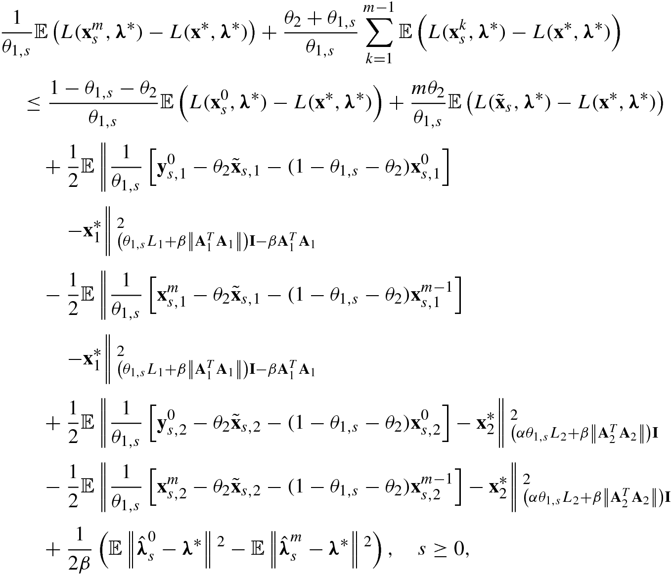
and  , respectively. Since L(x, λ
∗) is convex for x, we have
, respectively. Since L(x, λ
∗) is convex for x, we have ![$$\displaystyle \begin{aligned} &mL(\tilde{\mathbf{x}}_s,\boldsymbol\lambda^*)\\ &\quad =mL\left( \frac{1}{m}\left[\left(1-\frac{(\tau-1)\theta_{1,{s}}}{\theta_2} \right){\mathbf{x}}^m_{s-1}+\left(1+\frac{(\tau-1)\theta_{1,{s}}}{(m-1)\theta_2}\right)\sum_{k=1}^{m-1}{\mathbf{x}}^k_{s-1}\right],\boldsymbol\lambda^*\right)\\ &\quad \leq\left[1-\frac{(\tau-1)\theta_{1,{s}}}{\theta_2} \right]L({\mathbf{x}}^m_{s-1},\boldsymbol\lambda^*)+\left[1+\frac{(\tau-1)\theta_{1,{s}}}{(m-1)\theta_2}\right]\sum_{k=1}^{m-1}L({\mathbf{x}}^k_{s-1},\boldsymbol\lambda^*). \end{aligned} $$](../images/487003_1_En_5_Chapter/487003_1_En_5_Chapter_TeX_Equ180.png)
 , we have
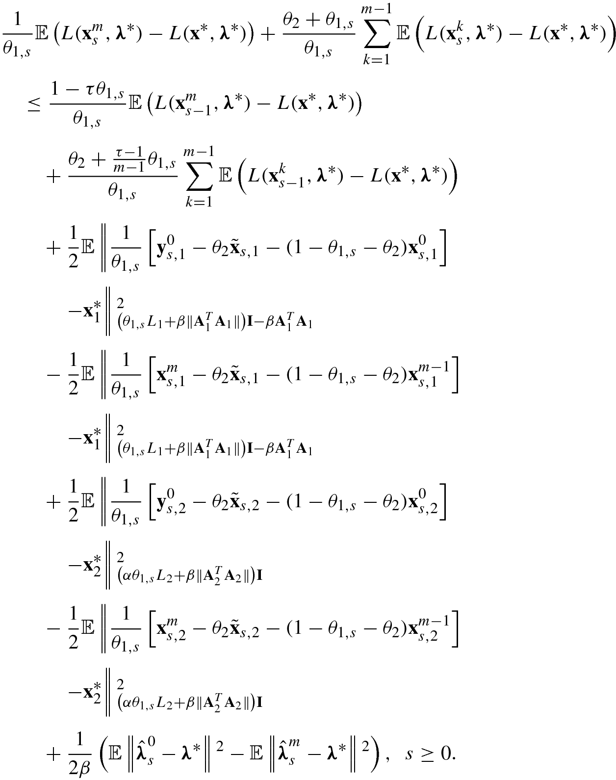
 and
and  , we have

![$$\displaystyle \begin{aligned} \begin{array}{rcl} {\mathbf{y}}_{s+1}^0&\displaystyle =&\displaystyle (1-\theta_2){\mathbf{x}}^m_s +\theta_2 \tilde{\mathbf{x}}_{s+1} \\ &\displaystyle &\displaystyle +\frac{\theta_{1,s+1}}{\theta_{1,s}}\left[(1-\theta_{1,s}){\mathbf{x}}^m_s-(1-\theta_{1,s}-\theta_2){\mathbf{x}}^{m-1}_s -\theta_2 \tilde{\mathbf{x}}_s\right], \end{array} \end{aligned} $$](../images/487003_1_En_5_Chapter/487003_1_En_5_Chapter_TeX_Equ185.png)
![$$\displaystyle \begin{aligned} \begin{array}{rcl}{} &\displaystyle &\displaystyle \frac{1}{\theta_{1,s}}\left[{\mathbf{x}}^{m}_s-\theta_2\tilde{\mathbf{x}}_s-(1-\theta_{1,s}-\theta_{2}){\mathbf{x}}^{m-1}_s\right]\\ &\displaystyle &\displaystyle \quad =\frac{1}{\theta_{1,s+1}}\left[{\mathbf{y}}^{0}_{s+1}-\theta_2\tilde{\mathbf{x}}_{s+1}-(1-\theta_{1,{s+1}}-\theta_{2}){\mathbf{x}}^{0}_{s+1}\right]. \end{array} \end{aligned} $$](../images/487003_1_En_5_Chapter/487003_1_En_5_Chapter_TeX_Equ186.png)
 , thus
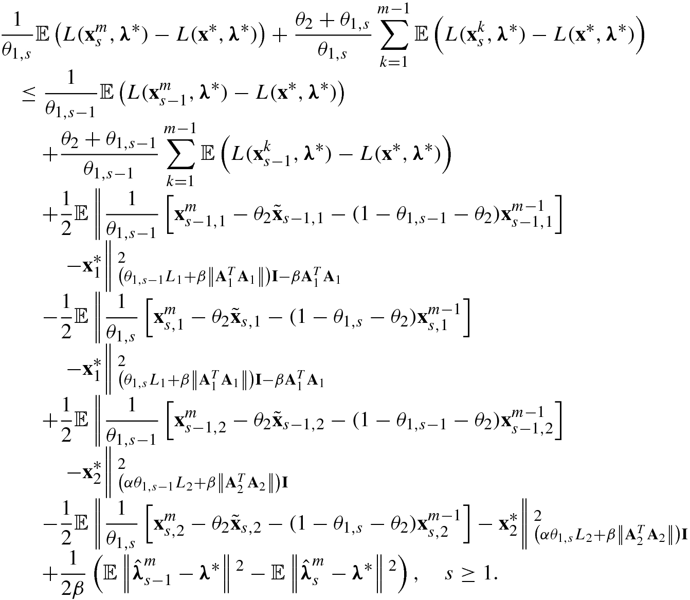
 ,
,  , and θ
1,0 ≥ θ
1,1, we obtain
, and θ
1,0 ≥ θ
1,1, we obtain 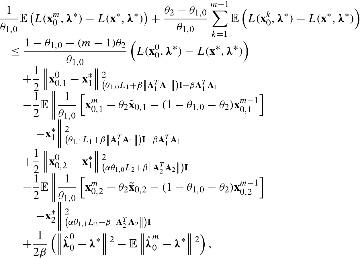
 . From (5.126), for s ≥ 1 we have
 ![$$\displaystyle \begin{aligned} \begin{array}{rcl}{} &\displaystyle &\displaystyle \hat{\boldsymbol\lambda}^{m}_s-\hat{\boldsymbol\lambda}^{m}_{s-1}=\hat{\boldsymbol\lambda}^{m}_s-\hat{\boldsymbol\lambda}^{0}_{s}= \sum_{k=1}^m \left(\hat{\boldsymbol\lambda}^{k}_s-\hat{\boldsymbol\lambda}^{k-1}_{s}\right)\\ &\displaystyle &\displaystyle \quad \overset{a}= \beta\sum_{k=1}^m \left[ \frac{1}{\theta_{1,{s}}} \left(\mathbf{A}{\mathbf{x}}^k_s-{\mathbf{b}}\right) - \frac{1-\theta_{1,{s}}-\theta_2}{\theta_{1,{s}}} \left(\mathbf{A}{\mathbf{x}}^{k-1}_s-{\mathbf{b}}\right) - \frac{\theta_2}{\theta_{1,{s}}} \left(\mathbf{A}\tilde{\mathbf{x}}_s-{\mathbf{b}}\right) \right]\\ &\displaystyle &\displaystyle \quad = \frac{\beta}{\theta_{1,s}}\left(\mathbf{A}{\mathbf{x}}^m_s-{\mathbf{b}}\right)+ \frac{\beta(\theta_2+\theta_{1,{s}})}{\theta_{1,s}}\sum_{k=1}^{m-1} \left(\mathbf{A}{\mathbf{x}}^k_s-{\mathbf{b}}\right)\\ &\displaystyle &\displaystyle \qquad -\frac{\beta(1-\theta_{1,s}-\theta_2)}{\theta_{1,s}}\left(\mathbf{A}{\mathbf{x}}^m_{s-1}-{\mathbf{b}}\right)- \frac{m\beta\theta_2}{\theta_{1,s}} \left(\mathbf{A}\tilde{\mathbf{x}}_{s}-{\mathbf{b}}\right)\\ &\displaystyle &\displaystyle \quad \overset{b}= \frac{\beta}{\theta_{1,s}}\left(\mathbf{A}{\mathbf{x}}^m_s-{\mathbf{b}}\right)+ \frac{\beta(\theta_2+\theta_{1,{s}})}{\theta_{1,s}}\sum_{k=1}^{m-1} \left(\mathbf{A}{\mathbf{x}}^k_s-{\mathbf{b}}\right)\\ &\displaystyle &\displaystyle \qquad -\beta\left[ \frac{1-\theta_{1,s}-(\tau-1)\theta_{1,{s}}}{\theta_{1,s}}\left(\mathbf{A}{\mathbf{x}}^m_{s-1}-{\mathbf{b}}\right)\right.\\ &\displaystyle &\displaystyle \qquad \left.+ \frac{\theta_{2}+\frac{\tau-1}{m-1}\theta_{1,{s}}}{\theta_{1,s}}\sum_{k=1}^{m-1}\left(\mathbf{A}{\mathbf{x}}^k_{s-1}-{\mathbf{b}}\right)\right]\\ &\displaystyle &\displaystyle \quad \overset{c}= \frac{\beta}{\theta_{1,s}}\left(\mathbf{A}{\mathbf{x}}^m_s-{\mathbf{b}}\right)+ \frac{\beta(\theta_2+\theta_{1,{s}})}{\theta_{1,s}}\sum_{k=1}^{m-1} \left(\mathbf{A}{\mathbf{x}}^k_s-{\mathbf{b}}\right)\\ &\displaystyle &\displaystyle \qquad -\frac{\beta}{\theta_{1,s-1}}\left(\mathbf{A}{\mathbf{x}}^m_{s-1}-{\mathbf{b}}\right)- \frac{\beta(\theta_2+\theta_{1,{s-1}})}{\theta_{1,s-1}}\sum_{k=1}^{m-1} \left(\mathbf{A}{\mathbf{x}}^k_{s-1}-{\mathbf{b}}\right), \end{array} \end{aligned} $$](../images/487003_1_En_5_Chapter/487003_1_En_5_Chapter_TeX_Equ190.png)
 uses (5.121),
  uses the definition of
  , and
, and  uses (5.139) and (5.140). When s = 0, we can obtain
 ![$$\displaystyle \begin{aligned} \begin{array}{rcl}{} \hat{\boldsymbol\lambda}^{m}_0-\hat{\boldsymbol\lambda}^{0}_{0}&\displaystyle =&\displaystyle \sum_{k=1}^m \left(\hat{\boldsymbol\lambda}^{k}_0-\hat{\boldsymbol\lambda}^{k-1}_{0}\right)\\ &\displaystyle =&\displaystyle \sum_{k=1}^m \left[ \frac{\beta}{\theta_{1,{0}}} \left(\mathbf{A}{\mathbf{x}}^k_0-{\mathbf{b}}\right) - \frac{\beta(1-\theta_{1,{0}}-\theta_2)}{\theta_{1,{0}}} \left(\mathbf{A}{\mathbf{x}}^{k-1}_0-{\mathbf{b}}\right)\right.\\ &\displaystyle &\displaystyle \left. - \frac{\theta_2\beta}{\theta_{1,{0}}} \left(\mathbf{A}{\mathbf{x}}^0_0-{\mathbf{b}}\right) \right]\\ &\displaystyle =&\displaystyle \frac{\beta}{\theta_{1,0}}\left(\mathbf{A}{\mathbf{x}}^m_0-{\mathbf{b}}\right)+ \frac{\beta(\theta_2+\theta_{1,{0}})}{\theta_{1,0}}\sum_{k=1}^{m-1} \left(\mathbf{A}{\mathbf{x}}^k_0-{\mathbf{b}}\right) \\ &\displaystyle &\displaystyle - \frac{\beta[1-\theta_{1,0}+(m-1)\theta_2]}{\theta_{1,0}}\left(\mathbf{A}{\mathbf{x}}^0_0-{\mathbf{b}} \right). \end{array} \end{aligned} $$](../images/487003_1_En_5_Chapter/487003_1_En_5_Chapter_TeX_Equ191.png)
![$$\displaystyle \begin{aligned} \begin{array}{rcl}{} \hat{\boldsymbol\lambda}^{m}_S-\boldsymbol\lambda^* &\displaystyle =&\displaystyle \hat{\boldsymbol\lambda}^{m}_S-\hat{\boldsymbol\lambda}^0_0 + \hat{\boldsymbol\lambda}^0_0 - \boldsymbol\lambda^*\\ &\displaystyle =&\displaystyle \frac{\beta}{\theta_{1,S}}\left(\mathbf{A}{\mathbf{x}}^m_S-{\mathbf{b}}\right)+ \frac{\beta(\theta_2+\theta_{1,{S}})}{\theta_{1,S}}\sum_{k=1}^{m-1} \left(\mathbf{A}{\mathbf{x}}^k_S-{\mathbf{b}}\right) \\ &\displaystyle &\displaystyle - \frac{\beta\left[1-\theta_{1,0}+(m-1)\theta_2\right]}{\theta_{1,0}}\left(\mathbf{A}{\mathbf{x}}^0_0-{\mathbf{b}} \right)\\ &\displaystyle &\displaystyle +\tilde{\boldsymbol\lambda}^{0}_0 +\frac{\beta(1-\theta_{1,{0}})}{\theta_{1,{0}}}\left(\mathbf{A}{\mathbf{x}}^0_{0}-{\mathbf{b}} \right) - \boldsymbol\lambda^*\\ &\displaystyle \overset{a}=&\displaystyle \frac{(m-1)(\theta_2+\theta_{1,S})\beta +\beta}{\theta_{1,{S}}}\left(\mathbf{A}\hat{\mathbf{x}}_S-{\mathbf{b}} \right) \\ &\displaystyle &\displaystyle +\tilde{\boldsymbol\lambda}^0_0 -\frac{\beta(m-1)\theta_2}{\theta_{1,{0}}}\left( \mathbf{A}{\mathbf{x}}^0_0 -{\mathbf{b}}\right) -\boldsymbol\lambda^*, \end{array} \end{aligned} $$](../images/487003_1_En_5_Chapter/487003_1_En_5_Chapter_TeX_Equ192.png)
 uses the definition of
  . Substituting (5.148) into (5.145) and using that L(x, λ) is convex in x, we have
 we can obtain (5.133). □
With Theorem 5.10 in hand, we can check that the convergence rate of Acc-SADMM
to solve problem (5.98) is exactly O(1∕(mS)). However, for non-accelerated methods, the convergence rate for ADMM
in the non-ergodic
sense is  [5].
[5].
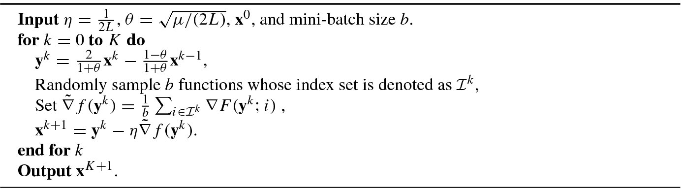
5.5 The Infinite Case
![$$\displaystyle \begin{aligned} \begin{array}{rcl}{} \min_{\mathbf{x}} f(\mathbf{x})\equiv \mathbb{E} [F(\mathbf{x};\xi)], \end{array} \end{aligned} $$](../images/487003_1_En_5_Chapter/487003_1_En_5_Chapter_TeX_Equ194.png)

We apply mini-batch AGD to solve (5.149). The algorithm is shown in Algorithm 5.8.


 . By taking the expectation on the random number in
  , we have
 we use
  . Thus we have
![$$\displaystyle \begin{aligned} \begin{array}{rcl} &\displaystyle &\displaystyle L\left\|{\mathbf{y}}^k -(1-\theta){\mathbf{x}}^k-\theta{\mathbf{x}}^*\right\|{}^2\\ &\displaystyle &\displaystyle \quad =\theta^2L\left\|\frac{1}{\theta}{\mathbf{y}}^k-\theta {\mathbf{x}}^*- \frac{1-\theta}{\theta}{\mathbf{x}}^k- (1-\theta){\mathbf{x}}^* \right\|{}^2\\ &\displaystyle &\displaystyle \quad =\theta^2L\left\|\theta ({\mathbf{y}}^k -{\mathbf{x}}^*) + \left(\frac{1}{\theta}-\theta\right){\mathbf{y}}^k - \frac{1-\theta}{\theta}{\mathbf{x}}^k- (1-\theta){\mathbf{x}}^* \right\|{}^2\\ &\displaystyle &\displaystyle \quad =\theta^2L\left\|\theta ({\mathbf{y}}^k -{\mathbf{x}}^*) + (1-\theta)\left[ \left(1+\frac{1}{\theta}\right){\mathbf{y}}^k -\frac{1}{\theta}{\mathbf{x}}^k -{\mathbf{x}}^* \right] \right\|{}^2\\ &\displaystyle &\displaystyle \quad \overset{a}\leq \theta^3L\left\|{\mathbf{y}}^k-{\mathbf{x}}^*\right\|{}^2 + \theta^2(1-\theta)L\left\| \left(1+\frac{1}{\theta}\right){\mathbf{y}}^k -\frac{1}{\theta}{\mathbf{x}}^k -{\mathbf{x}}^* \right\|{}^2\\ &\displaystyle &\displaystyle \quad \overset{b}=\frac{\theta\mu}{2}\left\|{\mathbf{y}}^k-{\mathbf{x}}^*\right\|{}^2 + \theta^2(1-\theta)L\left\| \left(1+\frac{1}{\theta}\right){\mathbf{y}}^k -\frac{1}{\theta}{\mathbf{x}}^k -{\mathbf{x}}^* \right\|{}^2, \end{array} \end{aligned} $$](../images/487003_1_En_5_Chapter/487003_1_En_5_Chapter_TeX_Equ203.png)
 we use the convexity of ∥⋅∥2 and in
  we use
  . Then from the update rule, we have
 ![$$\displaystyle \begin{aligned} \begin{array}{rcl} \frac{1}{\theta}\Big[{\mathbf{x}}^{k}-(1-\theta){\mathbf{x}}^{k-1}\Big] = \left(1+\frac{1}{\theta}\right){\mathbf{y}}^k -\frac{1}{\theta}{\mathbf{x}}^k. \end{array} \end{aligned} $$](../images/487003_1_En_5_Chapter/487003_1_En_5_Chapter_TeX_Equ204.png)

 and taking the first K iterations into account, we have
 mini-batch size, we have

Theorem 5.11 indicates that the total stochastic gradient calls is  . However, the algorithm converges in
  steps, which is the fastest rate even in deterministic algorithms. So the momentum technique enlarges the mini-batch size by
  times.