2 SELF-DRIVING CARS AND THE DARPA GRAND CHALLENGE

Most things worth doing aren’t easy, and they aren’t fast. You play with what you got, and how things turn out, that’s the way they are supposed to be. The right thing to do is choose something you love, go after it with everything you got, and that’s what life is about.

—William “Red” Whittaker, leader of the Red Team¹

THE $1 MILLION RACE IN THE DESERT

The first robot car race began in the Mojave Desert on a cool Thursday morning in 2004. As the sun began to rise, a desert tortoise poked its head out of its burrow, hoping to spend the day basking on the quickly warming road. Today he found himself trapped near his burrow, unable to move far in any direction. Some twenty biologists had put barriers around this and similar burrows to protect endangered species from the fleet of robot cars that was about to drive down the nearby highway.² They anticipated (correctly) that the cars wouldn’t be able to stay on the roads, let alone avoid tortoises in the middle of them.

Expectations about the cars’ ability to finish the race varied wildly. The race manager unblinkingly claimed a winner would finish the 142-mile span in under 10 hours.³ Others—including many in the robotics community—doubted that any contestants would finish the race at all.⁴

A $1 million prize was at stake. Among those who wanted that prize was Chris Urmson, design lead for a team of researchers developing a self-driving Humvee.

Chris was tall and thin, with messy blond hair. Under the mentorship of the legendary roboticist William “Red” Whittaker, Chris was working his way toward a PhD at Carnegie Mellon University (CMU). Singularly dedicated to his research, he had spent nearly two months in the desert running tests on the team’s Humvee, staying up for nearly 40 hours straight at one point.⁵ During one of its long-running tests he watched till near midnight, huddled under heavy blankets, as the Humvee drove in circles.⁶ With its headlights visible through the thin fog, the Humvee suddenly veered off-course into a chain-link fence.⁷ In another experiment the Humvee rolled over when it attempted a sharp turn, throwing its sensors off for weeks. Chris knew it was better to have these accidents before the race than during it.

A self-driving motorcycle was (of course) the media darling for the race. Its designers had attached gyroscopes to it so that it could remain upright by counter-turning just enough to stay balanced. It was among more than 100 submissions from researchers and hobbyists throughout the country.⁸ A gyroscopic motorcycle was clever, but everyone knew that if any team were to win the race it would likely be Chris and William’s team from CMU. Researchers from Carnegie Mellon had been leading the field for the past two decades, putting a rudimentary self-driving car onto Pittsburgh’s streets as far back as 1991. No one could deny the CMU researchers’ electromechanical chops. And their generous funding by military grants probably didn’t hurt.⁹

The day of the race, the Humvee designed by Chris and his team zoomed by the tortoise’s burrow, peppered with sensors and followed closely by another car. The Humvee had been driving for about 25 minutes. It wasn’t driving fast—it averaged a little over 15 miles per hour for the 7 miles it had traveled—but it was still faring better than the other submissions that day. Its windshield obscured by a large CAT logo, the robot car hummed along confidently. But suddenly its vision gave out as it followed a switchback curving sharply to the left. Unable to see the road, the car was driving blind.

HOW TO BUILD A SELF-DRIVING CAR

How did the Humvee drive on its own for seven miles? You might have heard that self-driving cars use machine learning—specifically “deep neural networks”—to drive themselves. But when Chris and his colleagues described their Humvee after the race, they didn’t mention machine learning or neural networks at all. This was 2004, nearly a decade before we had figured out how to train neural networks to reliably “see” objects. So what did these early self-driving cars use instead? In the next few chapters, I’ll answer this question, explaining some of the bare minimum algorithms that enable cars to drive autonomously. I’ll start by explaining how a car can drive for miles on a remote desert road without any traffic, when it has been given a list of locations to visit. Then I’ll work my way up over the next few chapters to describe the algorithms that enable these cars to “see” the world around them and to reason about driving in an urban environment well enough to obey California traffic laws. But before we get into those details—all of which are part of a self-driving car’s software—let’s take a quick look at the way a computer controls the hardware of the car.

When Vaucanson created the Flute Player we saw in the last chapter, he programmed it to play specific songs by carefully placing studs at specific locations on the rotating drum. These studs then pressed levers that controlled its lips, the airflow in its breath, and its fingers. IfVaucanson wanted to create a new song, he just needed to create a new drum with its studs placed at different locations. And if he wanted to change the way the statue moved its lips or fingers, while keeping his library of 12 songs, he just needed to adjust the levers, chains, and joints of the physical device. He had separated the development of his automaton into two parts—the rotating drum and the rest of the system—which made improving it and reasoning about it much easier. We can do the same thing with a self-driving car.

Let’s just focus on its speed for now. At its simplest, the car needs to turn a number the computer gives to it—such as “25”—into something concrete: the car’s driving speed. The thing that makes this more difficult than it sounds is that the physical engine has no concept of what “25” means. For example, even if you knew that applying 250 volts to an electric engine would make the car drive at 25 miles per hour, you couldn’t expect that by simply scaling the voltage up or down you’d get the speed you want. If you wanted the car to drive at one mile per hour, you couldn’t expect that applying 10 volts to the engine would do the job. It wouldn’t move at all at that voltage.

Vaucanson’s contemporaries solved this problem by using a device called a centrifugal governor, which creates a feedback loop to control the engine’s speed. A centrifugal governor is the “spinny” device with two metal balls—as shown in figure 2.1—that you might associate with steam engines and the mechanical workshops of the Enlightenment. As the engine runs faster, the governor spins more quickly, and the metal balls are pulled outward by centrifugal force. Through a series of levers, a valve closes on the fuel line feeding into the engine, slowing it back down. If the engine is running too slowly, the device increases fuel to the steam engine, speeding it back up. By adjusting the fuel to the engine, the governor keeps the engine’s speed consistent.

Figure 2.1

A centrifugal governor, the precursor to electronic control systems. As the engine runs more quickly, the rotating axis with the “flyballs” spins more rapidly, and the flyballs are pulled outward by centrifugal force. Through a series of levers, this causes the valve to the engine to close. If the engine is running too slowly, the valve will allow more fuel through.

The downside to this governor is that it only knows how to keep the engine running at a single speed. Modern self-driving cars use a similar feedback loop, except that they can run at whatever target speed is dictated by the computer program. You can see such a feedback loop in figure 2.2. Your target speed—say, 25 miles per hour—is an input to this feedback loop, and the loop uses an electronic speed sensor instead of a spinny device to gauge how far the wheel speed is from the target speed.

Figure 2.2

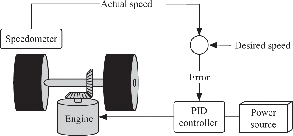
The control loop for a PID controller, the three-rule controller described in the text. The controller uses feedback from the speedometer to adjust inputs to the engine, such as power.

The intuitive behavior we want out of a speed control algorithm is that it will increase the power to the motor when the car is driving too slowly and decrease it when the car is driving too fast. One popular way to adjust the power to the motor is called proportional control, so-called because the adjustments we make to the power are equal to the difference between the target and current speed, multiplied by a fixed number. Proportional control isn’t perfect—if the car is driving uphill or driving against strong winds, it will tend to drive more slowly than we want. So usually a couple of other adjustments are made to the control algorithm—so that, for example, if the car is consistently too slow, the power to the engine will get a little boost. The most common control algorithm is a set of three simple rules like this that reliably get the car to its target speed. It was this three-rule controller (experts call it a PID controller) that was used in many of the self-driving cars we’ll cover in the next few chapters.¹⁰

Now that we have a rough sense for how to control the hardware, we don’t need to think a whole lot more about these messy details. Creating the hardware is certainly important, but we can assume that it’s a separate challenge, maybe a topic for a different book. To control speed and steering from our perspective, we just need to write software that tells the car what speed to drive at, and how much it should turn its wheels. We’ve turned driving a car from a hardware problem into a software problem, and now we can focus exclusively on that software problem.

PLANNING A PATH

When the Humvee drove in the race, it didn’t just drive for 25 minutes in a random direction; it drove along a path toward a specific destination. It did this because the car had a piece of software that told it where to go. This planning component is the most important part of the self-driving car: it determines the priorities for the rest of the system. Everything else the car does—such as steering to stay on the path and not crashing into rocks—is done to further the goal of following that path.

The organizers of the robot car race gave the contestants an electronic map of the route a mere two hours before the race started because they didn’t want the contestants to peek at the route. This map outlined—with global positioning system (GPS) coordinates—where the car could go on its way from the beginning of the race to the end of the race. So Chris and his team outfitted their car with a GPS sensor to detect where it was. In theory, the car simply needed to navigate from one spot on the map to another, using their GPS sensor to turn this way and that to stay close to the route.

Chris’s team, which called itself the Red Team, knew that GPS was the most important part of navigation, but they also knew that it wasn’t enough. Obstacles like fences and rocks would be in the way. So the Red Team also created a massive map in advance, which they called “the best map in the world,” to augment the one they would receive the morning of the race.¹¹ In the weeks before the race began, they studied satellite images from 54,000 square miles of desert to identify where the obstacles were located. Then, during the two-hour window in which they had the route’s GPS coordinates before the race started, fourteen humans hurried (with the help of a couple dozen computers) to manually annotate the terrain along the route.¹²

As these human workers annotated the map, a computer continuously searched for the best route from the start of the race to the end of it, sending updates back to the workers so they could prioritize their research. Chris and his team planned to upload this pre-computed path to their self-driving Humvee just before the race started.

PATH SEARCH

When you were a child, you may have played a game in which you pretended that the floor in your living room was hot lava. The point of this game was to find a path through the room that avoided the floor—that is, the lava—whenever possible. The Humvee needed to do the same thing to get from its current position to the next goal point in the map, except that instead of avoiding lava, it needed to avoid dangerous parts of the desert.

But we can’t simply tell the Humvee, “Find a good path.” Remember, when Vaucanson created the Flute Player, he had to provide the statue with instructions for every little movement it would need to make to play the flute. Similarly, when we program a computer to find a good path, we need to give it a clear sequence of steps it must follow to figure out that path on its own. These steps are like a recipe, except that we must be explicit about the most minute of details.

If we were to formalize the process you went through to find a path through your hot-lava living room, it probably went something like this. First, without thinking about it, you assigned a cost in your mind to taking a step on different surfaces or items in the room, perhaps like this:

Table 2.1

Terrain type		“Cost” of one step
Carpet (lava)		1
Table		0.5 (Mom will get mad, but it’s not lava)
Couch		0
Sleeping dog or cat		10

Then you planned your path through the room by estimating which sequence of steps would get you to the other side of the room for the least possible cost. Notice that we framed the problem of searching for a good path as minimizing some function (the cost of a path). This is important, because we framed the problem in terms of something computers are good at. They’re bad at open-ended planning in complex environments, but they’re good at minimizing functions. We will see this idea again and again in this book.

The Humvee was in a timed race, so the Red Team assigned a cost to each meter-by-meter cell in their map to reflect the time they expected the Humvee would take to safely drive one meter, on a six-point scale. Difficult terrain received a higher cost than easy terrain since the Humvee would need to drive more slowly on it. The team added extra penalties for regions of the map that were unpaved, lacked GPS data, or had uneven or steep ground, or for cells that were too far from the center of the race corridor described by their GPS coordinates. Once they had a map with costs assigned to each square cell, they needed to estimate their path through the map.

In one popular path-finding process called Dijkstra’s algorithm, the computer searches for a path by growing a search “frontier” out from the start point.¹³ The program runs a loop, pushing the frontier out a small amount each time it runs through the loop until eventually the frontier reaches the final destination. As the program grows the frontier, it slowly increases the cost it’s willing to “pay” to get to any point within the frontier; so any time it stretches the frontier to include another point, that new point is just at the cusp of what it’s willing to pay. The benefit of stretching the frontier like this is that the frontier can search along the most promising routes—such as smooth roads, which have a low cost—long before it bothers searching far into the more difficult routes—such as rough, off-road terrain.

By the time this frontier reaches the goal point—the destination, in the case of the self-driving car—the computer knows a path exists, and it knows the cost of that path. As long as the computer kept track of how it spread the frontier through the map, it can then quickly backtrack to find the shortest path to the goal point. You can see what such a shortest path looks like—as well as what the search frontier looks like—in figure 2.3.

Figure 2.3a

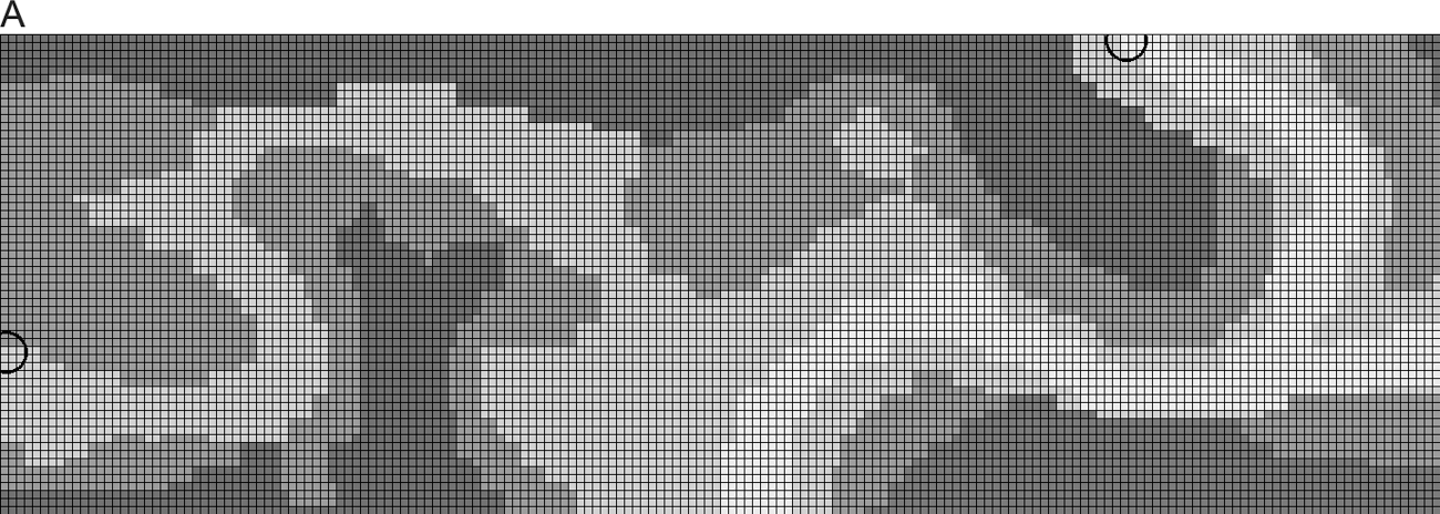
An example map. Darker shades indicate a higher travel cost.

Figure 2.3b

The search “frontier” at different iterations of Dijkstra’s algorithm.

Figure 2.3c

An optimal path through this map.

(a) A map with four different types of terrain. Each cell in the grid represents a square meter and takes one of four colors, indicating the type of terrain. Darker shades have a higher cost and cannot be traversed as easily. Start and end positions are respectively marked on the left and at the top. From lightest to darkest grey, the time to pass over a cell are 1.0, 3.0, 9.0, and 18.0 seconds / meter. (b) Some search algorithms run by growing a search “frontier” out from the start point. Each frontier is represented by a contour line; these represent how far the car could travel in 175, 350, 525, and 700 seconds. (c) Once the algorithm has completed, it has mapped an optimal path through the cost grid. In this case, the path tends to prefer to stay on light-colored terrain, on which the car can drive more quickly.

Computer scientists and roboticists have spent years studying algorithms like this, and they know how to find the lowest-cost path in large maps in a fraction of a second. When the path doesn’t need to be the best possible path—just a good-enough path—they can estimate it in even less time. After the Red Team’s computers planned the Humvee’s path with such an algorithm, the Humvee was ready to begin the race.

NAVIGATION

To find its position on the map, the Humvee used a GPS sensor that Chris’s team had strapped to it. GPS sensors use signals from a constellation of dozens of carefully calibrated satellites put into orbit by the US Department of Defense. At any given time, a handful of these satellites—not always the same ones—will be visible to a GPS sensor; it uses four of the visible ones to triangulate its current time (t) and its position (x, y, z) up to a few meters.

GPS alone isn’t enough for a self-driving car, however. First, GPS measurements aren’t consistently accurate: a good GPS system might be accurate up to centimeters, but some systems can be hundreds of meters off in the worst cases. There might also be gaps in GPS measurements from hardware hiccups, when passing through a tunnel, or even from disturbances of the satellites’ signals as the signals pass through the earth’s ionosphere. GPS also couldn’t tell the robot car its orientation: the Humvee might lose its bearings if its wheels slipped on the dusty road, for example. Having a way to navigate without GPS was therefore critical for the Humvee.

So the Red Team also put accelerometers onto the Humvee to measure its acceleration in three dimensions, which the Humvee accumulated to estimate the car’s velocity and position. They also attached gyros, which are accelerometers that measure rotation, so the Humvee could keep track of its orientation.

The car combined measurements from these accelerometers and GPS sensors using a Kalman filter, a mathematical model discovered in 1960. A Kalman filter is a method for tracking an object over time—the position of a submarine in the ocean or a robot Humvee, for example—by distilling a collection of measurements of the object into an estimate of its position. The core idea behind a Kalman filter is that we never really know an object’s true position and speed: we can only take imperfect snapshots, like blips on sonar. Some blips might be wrong, and we don’t want that to throw off the estimate—maybe it’s a reflection off of an orca or a piece of seaweed, for example—but a Kalman filter can smooth out these outliers. In fact, a Kalman filter doesn’t expect any of its measurements to be correct; it just expects them to be correct on average. And with enough observations, it can approximate an object’s true position and velocity extraordinarily well: a Kalman filter taking in measurements from accelerometers, gyros, and GPS, combined with measurements from the wheels, can enable a self-driving car to estimate its position, even during a two-minute GPS outage, with an error of mere centimeters.¹⁴

But even with these precise measurements, the Humvee might still run into fences, boulders, or other things along the road that might not have been visible in the Red Team’s map, so the team also added a gigantic “eye” to the Humvee. They planned for this giant eye to scan the ground in the Humvee’s path to find obstacles that weren’t already encoded into the preplanned route. If there were an object or uneven ground in the path it had intended to take, the Humvee was programmed to veer left or right to avoid hitting it.¹⁵

The eye was a combination of a laser and a light sensor, together called lidar, which is short for light detection and ranging. Lidar is like sonar or radar, except that it bounces light off objects instead of bouncing sound or radio waves off them. (I’ll use the term laser scanners from this point when I refer to the technology). The giant eye also had a pair of cameras mounted on a gimbal that could be pointed by the robot in different directions.¹⁶ (A gimbal is a fixture that enables an object to rotate along different axes, like that of a globe of the earth.)

But the Humvee’s giant eye was also very rudimentary. The Humvee wasn’t programmed to adjust its route in any material way in response to what its eye saw. It merely followed its preplanned path, veering left or right according to simple rules to avoid troublesome ground.

And this rudimentary eye was also what eventually gave the Humvee trouble, just before it skidded onto the shoulder of the road and crashed into a rock.

THE WINNER OF THE GRAND CHALLENGE

The Humvee hit the rock close to the place where we left it a few pages ago, just after passing its seven-mile mark in the desert. It had been following a switchback as it curved to the left, but the Humvee’s turn was too sharp, and its left wheels went over an embankment at the edge of the road. Its belly ground in the dirt as it slid forward until it hit the rock. A full minute on the race timer passed, followed by another, as the Humvee spun its wheels in the dust. A couple of race officials who had followed the Humvee to monitor its progress watched as the Humvee struggled in the morning light.

The Humvee’s tires spun for nearly seven minutes before finally catching fire. The nearby officials slammed a remote e-kill switch to stop the robot and jumped out to extinguish the flames. The Humvee’s wheels had been spinning so fast that both of its half-shafts split when they hit the kill switch.¹⁷ Chris’s team was officially out of the race.

A branch of the US Defense Department known as the Defense Advanced Research Projects Agency, or DARPA, organized this robot car race. Out of the 106 applicants to what became known as the DARPA Grand Challenge, 15 competed on the day of the race, including the robot Humvee designed by Chris and his team.

Exactly zero of these self-driving cars won the $1 million prize. To an onlooker, the competing cars might have looked like a rather pathetic bunch: one contestant, a large truck, slowly backed away from bushes, as another car, afraid of a shadow, drove off the road.¹⁸ The self-driving motorcycle’s creator, amid the excitement and cheering before the race, had forgotten to switch the motorcycle over to self-drive mode. It fell over at the starting line.¹⁹

The Humvee had driven 7.4 miles before grinding to a halt on the edge of the road. Although it was the race’s best performer, it had traveled a mere 5 percent of the route.

The Red Team studied their race logs and published a lengthy report outlining the strengths and weaknesses of their Humvee. In their report, they enumerated some problems during its 25-minute run. It reads like the script of a Blues Brothers movie:

Impact with fence post #1

Impact with fence post #2

Momentary pause

Impact with fence post #3

Impact with boulder

High centering in the hairpin [i.e., the final accident]²⁰

These impacts were described as “off-nominal behavior” in the Red Team’s report, but an insurance company might have more aptly called them “accidents.”

DARPA had announced to contestants that the race could be completed with a stock four-wheel-drive pickup truck,²¹ but the Red Team selected a Humvee because they didn’t want hardware to be a bottleneck. This did help in some cases. For example, fence post #3 was reinforced, which meant that the Humvee—which was more reinforced, as it was a Humvee—pushed against it for nearly two minutes before finally pushing it over and continuing on its way. Chris even called their Humvee a “battering ram of a car … at 22mph a Beast on a roll.”²² But a tough truck wasn’t enough to win.

The problem was that the Humvee could barely see where it was going. Its gigantic eye was too primitive, its vision too poor. Except for its ability to navigate over long distances, most of the Humvee’s intelligent behavior involved reacting to its sensors using simple rules. The Red Team, aware of these limitations, programmed the Humvee to ignore data from its camera and laser scanners when that data was likely to be unreliable, and then to follow its GPS coordinates, driving blind along its preplanned route. This is what happened right before the Humvee’s fatal crash. Its eye, and any software to support that eye, would have to be improved.

A FAILED RACE

To an outside observer, the Grand Challenge might have looked like a failure. CNN summarized it with the headline “Robots Fail to Complete Grand Challenge.”²⁸ Popular Science called it “DARPA’s Debacle in the Desert.”²³ On the bright side, as one spectator pointed out, it was “a good day for the tow-truck drivers.”²⁴

But many of the competitors were genuinely happy with the results. Contestants and organizers partied that night at Buffalo Bill’s Casino at the finish line, where they were surrounded by fellow geeks with a passion for building robot cars. Soon they would be able to read in detail about how a robot Humvee had managed to travel 7.4 miles—7.4 miles!—in rough desert terrain. They could also finally catch up on sleep after having worked nights and weekends for months.²⁵

DARPA officials were also excited, congratulating each other about the race. For the past eight years, the field of self-driving cars had been hibernating in virtual winter ever since Ernst Dickmanns, one of its leaders, had proclaimed that the field would need to wait until computers were more powerful. Now that computers were 25 times faster, DARPA’s Grand Prize had quickly begun to thaw the self-driving landscape so that researchers could make progress again.²⁶

DARPA was also a step closer to achieving its mandate from Congress—to make a third of military vehicles self-driving by 2015 (a mandate, to my knowledge, that they didn’t achieve). Like the contestants, DARPA had documentation from the world’s experts on how to make cars that could autonomously drive miles in the desert. “It didn’t matter to us if anybody completed the course,” DARPA director Anthony Tether explained. “We wanted to spark the interest in science and engineering in this area.”²⁷

Seen from that perspective, the race was a resounding success. It had attracted more than a hundred applicants and saw reporting from more than 450 television news segments and 58 newspapers within just a few months.²⁸ Top magazines like Wired and Popular Science featured the event in multipage spreads.²⁹ Although they didn’t know it at the time, it would also precede at least a decade and a half of heavy industry investment in self-driving car technology.

Eager to continue the progress, DARPA officials announced that they would hold another race in just over a year. They sweetened the prize, doubling the payout to $2 million. Gary Carr, one of the sleep-deprived contestants in the weeks leading up to the first challenge, was among those who could hardly wait. “We will be here. Our vehicle will be different, but we will be here.”³⁰ He wasn’t the only one excited about the next race. Chris and the rest of the Red Team now had another shot.