5 Nonlinear Data Structures: Trees

DOI: 10.1201/9781003105800-5

5.1 Basic Concept and Tree Terminology

5.1.1 Basic Concept

The tree is a nonlinear, non-primitive data structure. Trees are used in many applications to represent the relationship among the data elements that are nodes. Tree is a non-primitive, nonlinear data structure, which organizes data in a hierarchical design. In the tree data structure, every singular element is called a node. Each node in a nonlinear tree data structure stores the actual data of that particular element and the link part store address of the left or right sub-tree in a hierarchical manner. Tree data structure does not contain any cycle.

In a tree data structure, if we have N number of nodes, then we have a maximum of N-1 number of links or edges.

Example of tree:

5.1.2 Tree Terminology

1. Root node:

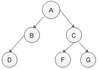
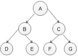
   In a tree data structure, the first node is called a root node. A parent-free node is referred to as a root node. Every tree needs a root node. The root node may be said to be the origin of the tree structure. In any tree data structure, there should be a single root node. We never have several root nodes within a tree. In Figure 5.1, ‘A’ is the root node of the tree.

   

   FIGURE 5.1 Tree with seven nodes and six links or edges.

2. Edge:

   In a tree data structure, the connecting link between any two nodes is called an edge. A tree with several nodes ‘N’ will have a maximum number of edges. In Figure 5.1, the link between nodes A and B is referred to as the edge.

3. Parent:

   In a tree data structure, the node which is the ancestor of any node is called the parent node. In simple terms, the node which has branched from it to any other node is known as the parent node. A parent node can also be described as, “the node that has a child or children”. In Figure 5.1. Nodes A, B and C are called parent nodes.

4. Child:

   In a tree data structure, the node that is a descendant of any node is referred to as a child node. In simple terms, the node that has an edge on its parent node is called the child node. Within a tree data structure, any parent node may have any number of child nodes. In a tree, all the nodes except the root are child nodes. In Figure 5.1, B, C, D, E, F and G are all child nodes.

5. Siblings:

   In a tree data structure, the nodes belonging to the same parent are referred to as brothers and sisters or siblings. In simple words, the nodes with the same parent are called sibling nodes. In Figure 5.1, B and C nodes are siblings of each other. In addition, nodes E, F and G are siblings of each other.

6. Leaf:

   In a tree data structure, the node with no child is called a leaf node. In simple terms, a leaf node is a node that has no child.

   In a tree data structure, leaf nodes are also known as external nodes. External node is also a node with no child. In a tree, a leaf node is also called a ‘Terminal’ node. In Figure 5.1, D, E, F and G are leaf nodes.

7. Internal nodes:

   The node that has at least one child is referred to as the internal node. In simple terms, an internal node is a node with at least one child.

   In a tree data structure, nodes other than leaf nodes or external nodes are called internal nodes. The root node is also considered an internal node if the tree structure has more than one node. Internal nodes are also called non-terminal nodes. In Figure 5.1, A, B and C nodes are the internal nodes.

8. Degree:

   In a nonlinear tree data structure, the total number of children of a node is known as the degree of that node. Simply stated, the degree of a node in a tree data structure is the total number of child nodes it has.

   The highest degree of a node among all the nodes of a tree is termed as ‘degree of tree’. In Figure 5.1, the degree of the C node is 3 and the degree of the B node is 1. However, the degree of tree is 3.

9. Level:

   In a nonlinear tree data structure, the root node is stated to be at Level 0 and the children of the root node are at Level 1 and the children of the nodes which are at Level 1 will be at Level 2 and so on. Simply stated, in a tree data structure, each step from top to bottom is called a Level, and the Level count starts with ‘0’ and is incremented by one at each level or step. In Figure 5.1, levels of D, E, F and G are 2.

10. Height:

    In a nonlinear tree data structure, the total number of edges or links from a leaf node to a specific node in the longest path is called as height of that node. In a tree, the height of the root node is said to be the height of the tree. In a tree, the height of all leaf nodes is ‘0’.

    In Figure 5.1, the height of the A node is 2 and the height of tree is also 2.

11. Depth:

    In a nonlinear tree data structure, the total number of edges from the root node to a particular node is called the depth of that node. In a tree, the total number of edges from the root node to a leaf node in the longest path is said to be the depth of the tree. Simply stated, the highest depth of any leaf node in a tree is said to be the depth of that tree. In a tree, the depth of the root node is ‘0’.

    In Figure 5.1, the depth of node D is 2 and the depth of a tree is also 2. The height and depth of a tree are equal, but the height and depth of the node are not equal because the height is calculated by traversing from a given node to the deepest possible leaf node. Depth is calculated from traversing from root to the given node.

12. Path:

    In a nonlinear tree data structure, the sequence of nodes and edges from one node to another node is called a path between the two nodes. The length of a path represents the total number of nodes on that path. In Figure 5.1, path A - B - D has length 3.

13. Sub-tree:

    In a nonlinear tree data structure, each child of a node forms a subtree recursively. Each child node consists of a sub-tree with its parent node.

14. Forest:

    Forest is the disjoint union of trees.

5.2 Data Structure for Binary Trees

5.2.1 Binary Tree Definition with Example

A tree in which each node can have a maximum of two children is called a binary tree. The degree of each node in the binary tree will be at most two (Figure 5.2).

FIGURE 5.2 Binary tree.

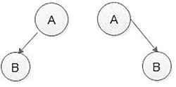
A binary tree with only one node is a binary tree with a root in which the left and right sub-trees are empty. If there are two nodes in a binary tree, one will be the root and another can be either the left or the right child of the root (Figure 5.3).

FIGURE 5.3 Two binary trees with two nodes.

5.2.2 Types of Binary Tree

1. Strictly binary tree or full binary tree or proper binary tree:

   A full binary tree or a proper binary tree or a strictly binary tree is a tree in which each node other than the leaves has two children. This means each node in the binary tree will have either 0 or 2 children is said to be a full binary tree or strictly binary tree. A complete binary tree is used to depict mathematical expressions (Figure 5.4).

   

   FIGURE 5.4 Strictly binary tree or full binary tree or proper binary tree.

2. Complete binary tree or perfect binary tree:

   A complete binary tree is a binary tree in which every level, except possibly the last, is filled, and all nodes are as far left as possible. All complete binary trees are strictly binary trees, but all strictly binary trees are not complete binary trees. A complete binary tree is the first strictly binary tree with the height difference of only 1 allowed between the left and right sub-tree. All leaf nodes are either at the same level or only a difference of 1 level is permissible (Figure 5.5).

   

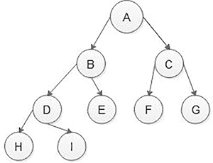
   FIGURE 5.5 Complete binary tree.

3. Binary search tree:

   If a binary tree has the property that all elements in the left sub-tree of a node n are lesser than the contents of n and all elements in the right sub-tree are greater than or equal to the contents of n, such a binary tree is called a binary search tree (BST).

   In a BST, if the same elements are inserted, then the same element is inserted on the right side of the node, having the same value. A BST is shown in Figure 5.6.

   

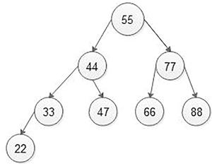
   FIGURE 5.6 Binary search tree.

4. Almost complete binary tree:

   A binary tree of depth d is called an almost complete binary tree if and only if:

1. Each leaf node in the tree is either at level d or at level d-1, which means the difference between levels of leaf nodes is only one is permissible.
2. At depth d, that is the last level, if a node is present, then all the nodes to the left of that node should also be present first, and no gap between the two nodes from the left to the right side of level d.

   In Figure 5.7, nodes at the last level are filled from left to right, and no gaps between the last level’s nodes. However, in Figure 8, the last level, having two nodes H and I have one gap because D nodes left child is present, but the right child is absent so Figure 5.8 is not an almost complete binary tree.

   

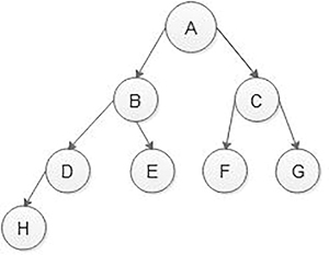
   FIGURE 5.7 Almost complete binary tree.

   Figure 5.7 shows almost a complete binary tree, but not a complete binary tree because the D node has a left child but no right child. In the complete binary tree, every interior node has exactly two children.

3. Skewed binary tree:

   If a tree is dominated by the left child node or the right child node, it is said to be a skewed binary tree.

   

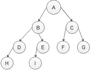
   FIGURE 5.8 Not an almost complete binary tree.

   In a left-skewed tree, most of the nodes have a left child without a corresponding right child as shown in Figure 5.9. In a right-skewed tree, most of the nodes have the right child without a corresponding left child as shown in Figure 5.10.

   

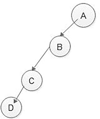
   FIGURE 5.9 Left skewed tree.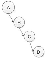

   

   FIGURE 5.10 Right skewed tree.

5.2.3 Binary Tree Representation

There are two binary tree representation techniques:

1. Sequential representation or array representation
2. Linked representation or linked list representation

5.2.3.1 Sequential Representation or Array Representation

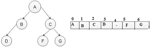
If a binary tree is a complete binary tree and if the depth of a tree is 3, then the total number of nodes is 7. That is, if the complete binary tree has depth n, then max nodes are calculated by 2n − 1 (Figure 5.11).

FIGURE 5.11 Complete binary tree.

If the depth of a binary tree is known, then we can represent binary trees using an array data structure. In sequential representation, the numbering of each node will start from the root node, and then the remaining nodes will give ever-increasing numbers in a level-wise direction. The nodes on the same level will be numbered from left to right. The numbering will be as shown in Figure 5.12.

FIGURE 5.12 Sequential representation of binary tree using array.

If we know the index of parent node suppose n, then its left child node is represented as,

Left child (n) = (2n+1)

If we know the index of parent node suppose n, then its right child node is represented as,

Right child (n) = (2n+2)

Here, root node is at index 0.

In Figure 5.12, node C is at index 2, then its left child is at index 5 and the right child is at index 6. In addition, if we know the index of the left child, then we can calculate the index of its parent node using formula (n-1)/2, and if we know the index of the right child, then we can calculate the index of its parent node using formula (n-2)/2.

Advantages of sequential representation:

1. Direct access to any node can be possible.
2. Finding parent or finding left, the right child of any particular node is faster.

Disadvantages of sequential representation:

1. Wastage of memory: If a binary tree is not a complete binary tree, then array size increased. For example, in Figure 5.12, the depth of a tree is 3, then the maximum size of the array is 2³ – 1, that is, 7, but actual array utilization is 6.
2. In this type of representation, prior knowledge of the depth of a tree is required because on that basis we have to fix the size of the array.
3. Insertion and deletion of any node in the tree will be costlier as other nodes have to be adjusted at appropriate positions. Therefore, the meaning of a binary tree can be preserved. As there are the abovementioned drawbacks in the sequential representation, we will search for a more flexible representation. Therefore, instead of the array, we will make use of linked list representation to represent a binary tree.

5.2.3.2 Linked List Representation

In linked list representation, each node will look like this (Figure 5.13):

FIGURE 5.13 Node in the linked list representation.

Left Child

Data

Right Child

The C structure for nodes in the binary tree is as follows:

struct binary_tree
{
struct bt *left;
int data;
struct bt *right;
};

Advantages of Linked list representation:

1. There is no wastage of memory.
2. There is no need to have prior knowledge of the depth of the tree. Using the dynamic memory management concept, we can create as much memory or nodes as required.
3. Insertion and deletion of nodes that are the most common operations can be done without moving other nodes.

Disadvantages of Linked list representation:

1. This representation gives no direct access to a node, and special algorithms are required.
2. This representation needs additional space in each node to store left and right sub-tree addresses.
3. The direct address of the left and right child does not get in linked representation.

5.2.4 Operations on Binary Tree

1. To create a binary tree.
2. To display data in each node of binary tree that is tree traversal.
3. To insert any node in the binary tree as the left child or right child of any node.
4. To delete a node from a binary tree.

5.2.5 Binary Tree Traversals

Traversing the tree means visiting each node in the tree exactly once. There are six ways to traverse a tree. For these traversals, we will use some notations as:

1. L means move to left child.
2. R means move to right child.
3. R’ means move to root or parent node.

Therefore, there are six different combinations of L, R, R’ nodes as LR’R, LRR’, R’LR, R’RL, RR’L and RLR’.

However, from there three traversing methods are important, which are as follows:

1. Left-Root-Right (LR’R): In-order traversal.
2. Root-Left-Right (R’LR): Preorder traversal.
3. Left-Right-Root (R’LR): Post-order traversal.

These all above traversing technique is also called as Depth First searching (DFS) or Depth First Traversal.

A tree is typically traversed in two ways:

1. Breadth first traversal (BFS) or level order traversal
2. Depth first traversal (DFS)

5.2.5.1 Breadth First Traversal or Level Order Traversal

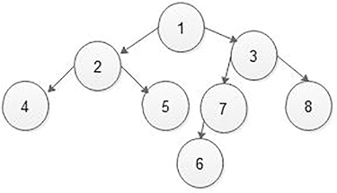
In the above traverse method, the items are visited level-wise. Therefore, the first node A is visited, then at the second level, first the nodes B then C are visited, and then at the third level, first nodes D, then F and then G are visited (Figure 5.14).

FIGURE 5.14 Binary tree traverse by using Breadth First Traversal or Level Order Traversal.

Level Order Traversal is as follows: A - B - C - D - F – G

Algorithm

In a binary tree, the root node is visited first, then its child nodes are visited and enqueue in a queue. Then dequeue a node from the queue and find its child nodes and again insert it into queue till all nodes are visited.

Algorithm for Level Order Traversal in Binary tree

1. Create an empty queue q.
2. temp_node = root // Start from the root node and assign the value of root to temp_node
3. while temp_node is not NULL repeat the steps
   1. 3.1 Print temp_node->data.
   2. 3.2. Enqueue temp_node’s children from first left then right children to q.
   3. 3.3. Dequeue a node from q and assign its value to temp_node.
4. Stop.

Time Complexity of Breadth First Traversal or Level Order Traversal: O (n) because we visit every node exactly once.

Extra space required for level order traversal is O (w) where w is the maximum width of a binary tree. In breadth first traversal, a queue data structure is required. In breadth first traversal, queue data structure stores one by one node of different levels.

5.2.5.2 Depth First Traversal

Depth first traversal has following three types of traversing:

1. In-order traversal
2. Preorder traversal
3. Post-order traversal

5.2.5.2.1 In-order Traversal

The basic principle is to traverse the left sub-tree, then root and then the right sub-tree (Figure 5.15).

FIGURE 5.15 Binary tree traverse by using in-order traversal method.

In-order traversal is as follows: D - B - A - F - C – G

5.2.5.2.2 Preorder Traversal

The basic principle is to traverse the first root, then the left sub-tree and then the right sub-tree (Figure 5.16).

FIGURE 5.16 Binary tree traverse by using preorder traversal method.

Preorder traversal is as follows: A - B - D - C - F – G

5.2.5.2.3 Post-order Traversal

The basic principle is to traverse the first left sub-tree, then the right sub-tree and then root (Figure 5.17).

FIGURE 5.17 Binary tree traverse by using post-order traversal method.

Post-order traversal is as follows: D - B - F - G - C – A

5.2.6 Simple Binary Tree Implementation

Creating a simple binary tree, the first element will form the root node. For all the next elements, the user has to enter whether that element has to be inserted as a left child or a right child of the previous node.

Example:

Let us say 10 is the root node,

If the next node says 21, then users will be asked for his choice that is attached to the left or right of 10. If the user answers left or l, then the tree will be,

Then, if the next element is 11, then again the user has to give his choice, whether it is left or right. That means first whether the user wants to attach 11 left or right of root 10. Then, if the user answers left, then again the user asks whether the user wants to attach 11 to left or right of 21, and if the user answers right, then node 11 will be attached as a right child of 21.

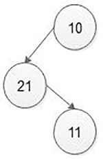
Thus, a simple binary will be generated. The principal idea behind this creation is to always ask the user where he wants to attach the next node and always start scanning the tree from the root.

Program: Implementation of simple binary tree and performing recursive insertion and traversing operations on a simple binary tree.

#include<stdio.h>
#include<stdlib.h>
struct bt
{
struct bt *left;
int data;
struct bt *right;
};
// Function prototypes
void insert(struct bt *root, struct bt *new1);
void in-order(struct bt *temp);
void preorder(struct bt *temp);
void postorder(struct bt *temp);
// main function definition

int main()
{
struct bt *root, *new1;
int ch;
char c;
root=NULL;
do
{
printf("1. Create 2.In-order 3. Preorder 4. Postorder 5. Exit \n");
printf("Enter your choice: ");
scanf("%d",&ch);
switch(ch)
{
case 1:
do
       {
       new1=(struct bt*)malloc(sizeof(struct bt));
       printf("\n Enter data: ");
       scanf("%d",&new1->data);
       new1->left=NULL;
       new1->right=NULL;
       if(root==NULL)
       {
       root=new1;
       }
       else
       {
       insert(root,new1);
       }
       printf("\n Do you want to insert new node [y/n]: ");
       c = getche();
       }while(c=='y'||c=='Y');
       break;
case 2:
       if(root==NULL)
       printf("\n Binary Tree is not created");
       else
       {
       in-order(root);
       }
       break;
case 3:
       if(root==NULL)
       printf("Binary Tree is not created");
       else
       {

       preorder(root);
       }
       break;
case 4:
       if(root==NULL)
       printf("Binary Tree is not created");
       else
       {
       postorder(root);
       }
       break;
case 5:
      exit(0);
default:
      printf("\n wrong choice: ");
}
printf("\n Do you want to continue Binary Tree [y/n] : ");
fflush(stdin);
scanf("%c",&c);
}while(c=='y'||c=='Y');
return 0;
}
void insert(struct bt* root, struct bt *new1)
{
char c;
printf("\n Where to insert node right or left of %d  : ",
root->data);
c=getche();
//if new node is to be inserted at right sub-tree
if(c=='r'||c=='R')
{
   if(root->right==NULL)  //if root node's right pointer is
   NULL then insert new node to
                                           // right side
   {
   root->right=new1;
   }
   else                // otherwise call insert function
   recursively 
   {
   insert(root->right,new1);
}
}
//if new node is to be inserted at left sub-tree
if(c=='l'||c=='L')
{
if(root->left==NULL)

{
root->left=new1;
}
else
{
insert(root->left,new1);
}
}
}
//in-order traversing of a simple binary tree
void in-order(struct bt *temp) //pass root node address as an
argument to a in-order function
{
if(temp != NULL)
{
in-order(temp->left); // Traverse the left sub-tree of root
R
printf("%d\t", temp->data);  //Visit the root, R and display.
in-order(temp->right);  //Traverse the right sub-tree of root
R
}
}
//preorder traversing of a simple binary tree
void preorder(struct bt *temp) //pass root node address as an
argument to a preorder 
                                                        //
      function
{
if(temp != NULL)
{
printf("%d\t", temp->data); //Visit the root, R and display.
preorder(temp->left); // Traverse the left sub-tree of root
R
preorder(temp->right); //Traverse the right sub-tree of root
R
}
}
//post-order traversing of a simple binary tree
void postorder(struct bt *temp) //pass root node address as an
argument to post-order 
                                //function
{
if(temp!=NULL)
{
postorder(temp->left);  // Traverse the left sub-tree of root R
postorder(temp->right); //Traverse the right sub-tree of root R
printf("%d\t",temp->data); //Visit the root, R and display.
}
}

Output:

5.3 Algorithms for Tree Traversals

5.3.1 Recursive Algorithm for In-order Traversal

In-order traversing of a binary tree T with root R.

Algorithm in-order (root):

1. Traverse the left sub-tree of root R, that is, call in-order (left sub-tree).
2. Visit the root, R and process.
3. Traverse the right sub-tree of root R, that is, call in-order (right sub-tree).

5.3.2 Recursive Algorithm for Preorder Traversal

Preorder traversing of binary tree T with root R.

Algorithm preorder (root):

1. Visit the root, R and process.
2. Traverse the left sub-tree of root R, that is, call preorder (left sub-tree)
3. Traverse the right sub-tree of root R, that is, call preorder (right sub-tree)

5.3.3 Recursive Algorithm for Postorder Traversal

Postorder traversing of binary tree T with root R.

Algorithm Postorder (Root)

1. Traverse the left sub-tree of root R, that is, call postorder (left sub-tree)
2. Traverse the right sub-tree of root R, that is, call postorder (right sub-tree)
3. Visit the root, R and process.

5.4 Construct a Binary Tree from Given Traversing Methods

5.4.1 Construct a Binary Tree from Given In-order and Preorder Traversing

Take one example:

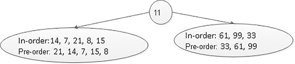
1. In-order traversal: 14, 7, 21, 8, 15, 11, 61, 99 and 33
2. Preorder traversal: 11, 21, 14, 7, 15, 8, 33, 61 and 99

The first value in the preorder traversal is the root of the binary tree because in preorder traversing, the first root is traversed, then the left sub-tree and then the right sub-tree is traversed. Therefore, the node with data 11 becomes the root of the binary tree. In in-order traversal, initially, the left sub-tree is traversed, then the root node and then the right sub-tree. Therefore, the data before 11 in the in-order list, that is, 14, 7, 21, 8 and 15 forms the left sub-tree, and the data after 11 in the in-order list, that is, 61, 99 and 33 forms the right sub-tree. Figure 5.18 shows the structure of the tree after dividing the tree into left and right sub-trees.

FIGURE 5.18 Reconstruction of a binary tree step 1.

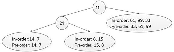
In the next iteration, 21 is the root for the left sub-tree. Hence, the data before 21 in the in-order list, that is, 14, 7 form the left sub-tree of the node that contains a value 21. The data that come to the right of 21 in the in-order list that is 8, 15 forms the right sub-tree of the node with value 21. Figure 5.19 shows the structure of the tree after expanding the left and right sub-tree of the node that contains a value 21.

FIGURE 5.19 Reconstruction of a binary tree step 2.

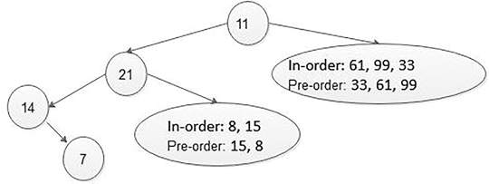
Now the next data in the preorder list is 14 so now it becomes the root node. The data before 14 in the in-order list forms the left sub-tree of the node that contains a value 14. However, as there is no data present before 14 in in-order list, the left sub-tree of the node with value 14 is empty. The data that come to the right of 14 in the in-order list is 7 forms the right sub-tree of the node that contains a value 14. Figure 5.20 shows the structure of the tree after expanding the left and right sub-tree of the node that contains a value 14.

FIGURE 5.20 Reconstruction of a binary tree step 3.

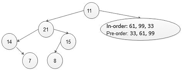
In the same way, one by one all the data are picked from the preorder list and are treated as root and then from in-order list find elements in the right and left sub-tree, and the whole tree is constructed in a recursive way or non-recursive way, that is, iterative way (Figures 5.21 and 5.22).

FIGURE 5.21 Reconstruction of a binary tree step 4.

FIGURE 5.22 Reconstruction of a binary tree step 5.

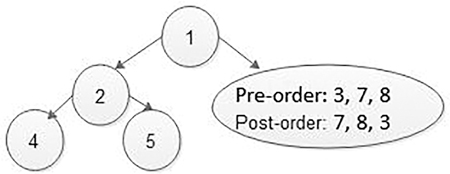
5.4.2 Construct a Binary Tree from Given In-order and Post-order Traversing

Take an example:

1. In-order traversal: 4 2 5 1 6 7 3 8
2. Post-order traversal: 4 5 2 6 7 8 3 1

The last value in the post-order traversal is the root of the binary tree because in post-order traversing root is traversed in the last then the left sub-tree and then the right sub-tree is traversed. Therefore, the node with data 1 becomes the root of the binary tree. In in-order traversal, initially the left sub-tree is traversed, then the root node and then the right sub-tree. Therefore, the data before 1 in the in-order list that is 4, 2, 5 forms the left sub-tree and the data after 1 in the in-order list that is 6, 7, 3, 8 forms the right sub-tree. Figure 5.23, shows the structure of the tree after dividing the tree into the left and right sub-trees.

FIGURE 5.23 Reconstruction of a binary tree step 1.

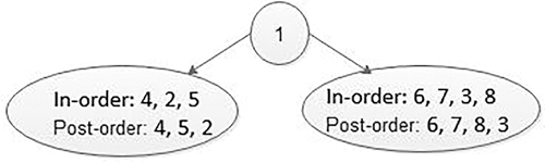
In the next iteration 2 is root for the left sub-tree because it is the last element in post-order traversing. Hence, the data before 2 in the in-order list that is 4 forms the left sub-tree of the node that contains a value 2. The data that comes to the right of 2 in the in-order list that is 5 forms the right sub-tree of the node with value 2. Figure 5.24 shows the structure of the tree after expanding the left and right sub-tree of the node that contains a value 2.

FIGURE 5.24 Reconstruction of a binary tree step 2.

In the same way, one by one last data elements are picked from the post-order list and are treated as root, and then from the in-order list find elements in the right and left sub-tree and the whole tree is constructed in a recursive way or non-recursive way (Figures 5.25 and 5.26).

FIGURE 5.25 Reconstruction of a binary tree step 3.

FIGURE 5.26 Reconstruction of a binary tree step 4.

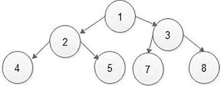
5.4.3 Construct a Strictly or Full Binary Tree from Given Preorder and Post-order Traversing

If we have preorder and post-order traversing sequence, then we cannot form or construct simple or general binary tree. Because for two different binary trees post and preorder traversing the sequence may be the same as shown in Figure 5.27.

FIGURE 5.27 Binary tree.

1. Preorder traversal: 1 - 2 - 3
2. Post-order traversal: 3 - 2 - 1

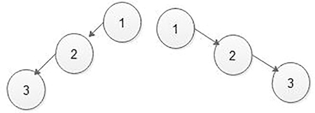
In Figure 5.27a and b, both preorder and post-order traversal give us the same result. That is, using preorder and post-order traversal, we cannot predict exactly which binary tree we want to construct. That means ambiguity is there.

However, if we know that the binary tree is strictly or a full binary tree, we can construct the binary tree without ambiguity.

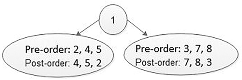
Take an example:

1. Preorder traversal: 1 2 4 5 3 7 8
2. Post-order traversal: 4 5 2 7 8 3 1

The last value in the post-order traversal is the root of the binary tree. The first value in preorder traversal is also root. Therefore, the node with data 1 becomes the root of the binary tree. The value next to 1 in preorder, must be left child of the root. Therefore, we know 1 is root and 2 is the left child. Now we know 2 is the root of all nodes in the left sub-tree. All nodes before 2 in post-order must be in the left sub-tree that is 4, 5 and 2. Now we know 1 is the root, elements 4, 5 and 2 are in the left sub-tree, and the elements 7, 8 and 3 are in the right sub-tree (Figures 5.28 and 5.29).

FIGURE 5.28 Reconstruction of a full binary tree step 1.

FIGURE 5.29 Reconstruction of a full binary tree step 2.

In the same way, one by one last data elements are picked from the post-order list and are treated as root and then from in-order list find elements in the right and left sub-tree, and the whole tree is constructed either in a recursive way or in a non-recursive way, i.e., iterative way (Figure 5.30).

FIGURE 5.30 Reconstruction of a full binary tree step 3.

5.5 Binary Search Trees

5.5.1 Basic Concepts of BSTs

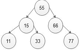
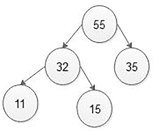
In a simple binary tree, nodes are located in any fashion. According to the user’s aspiration, new nodes can be connected as a left or right child of any desired node. In such a case, finding for any node is a long cut procedure because we have to search the entire tree. In addition, the complexity of the search time is going to increase unnecessarily. Therefore, to make the search algorithm quicker in a binary tree, let us create the BST. The BST is derived from a binary search algorithm. During the creation of a BST, the data are systematically organized. That means, the value of the left sub-tree < root node < value at the right sub-tree (Figure 5.31).

FIGURE 5.31 Binary search trees.

5.5.2 Operations on BSTs

1. Insertion of nodes in the BST
2. Deletion of a node from BST
3. Searching for a particular node in BST

Let us discuss these operations with examples:

5.5.2.1 Insertion of Node in the BST

While inserting any node in BST, first of all, we have to look for its appropriate position in BST.

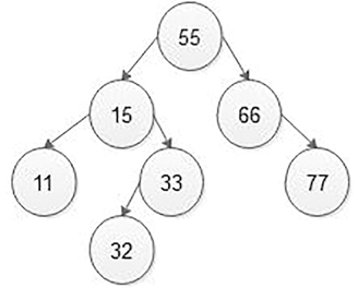
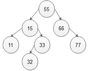
In Figure 5.32, if we want to insert 32, then we will start comparing 32 with a value of root, that is, 55. As 32 is less than 55, we will move on the left sub-tree. Now we will compare 32 with 15, and 32 is greater than 15 so move on the right sub-tree. Again, compare 32 with 33, and 32 is less than 33 so move to left sub-tree, but the left sub-tree is empty, so attach 32 nodes on the left side of 33 nodes as the left child of 33 nodes (Figure 5.33).

FIGURE 5.32 Before insertion of a node in the binary search tree.

FIGURE 5.33 After insertion of node 32 in a binary search tree.

5.5.2.2 Deletion of Node in the BST

For deleting a node from a BST, there are three possible cases:

1. Deletion of the leaf node from a BST
2. Deletion of a node having one child as left or right
3. Deletion of a node having two children.

5.5.2.2.1 Deletion of a Leaf Node

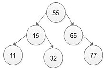
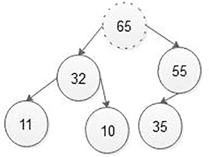
This is the simplest deletion, in which we first search the node which we want to delete and its respective parent. If the node which we want to delete is a leaf node, then that leaf node is either left or right child of its respective parent, then set the left or right pointer of the parent node as NULL (Figure 5.34) (Figure 5.34).

FIGURE 5.34 Before deletion of a leaf node from binary search tree.

In the above BST, the node having value 33 is a leaf node, that node we want to delete means that we will first search the node 33 in the BST and find its parent node that is 15. Then find 33 nodes are left or right side of the 15-parent node. In the above example, 33 nodes are on the right side of parent node 15 so make 15 node’s right pointer as NULL. In addition, free the node 33 as is shown in Figure 5.35.

FIGURE 5.35 After deletion of node 33 from binary search tree.

5.5.2.2.2 Deletion of a Node Having One Child as Left or Right

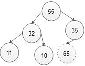
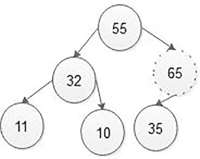
If the node which we want to delete from the BST is an interior node having one right child, then find its parent node and check whether that deleted node is a left or right child of the parent node. If the deleted node is the right child of the parent node, then copy the address of the right child of the deleted node into the right side of the parent node (Figure 5.36).

FIGURE 5.36 Before deletion.

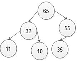
We want to delete node 33 in the above BST because it has an only left child. To do so, we will first search node 33 in the BST and find its parent node, that is, 15. Then find if the 33 node is on the left or right side of the 15 parent node. In the above example, 33 node is at the right side of parent node 15 so copy the address of the left child of deleted node 33 to the right side of parent node 15. Then set deleted node as free from BST as is shown in Figure 5.37.

FIGURE 5.37 After deletion of node 33 from binary search tree.

5.5.2.2.3 Deletion of a Node Having Two Children

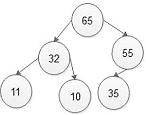
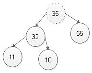
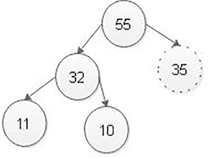
If the node which we want to delete from the BST is an interior node having two children, then find its parent node and in-order successor of the node which we want to delete. Then simply replace the in-order successor node value by deleting the node value. Then free the in-order successor node of the BST. In-order successor means to traverse the BST from a deleted node in the in-order traversing method and find the next element after deleting an element that is your in-order successor. Now take an example:

Because the node with the value 15 has two children in the above BST, the node 15 that we want to delete means will first be searched in the BST for its parent node, which is 55. Then find its in-order successor that is shown in Figure 5.38, 15 node’s in-order successor is 15, 32 and 33. That is the in-order successor of 15 nodes is 32 so replace 15 node value by 32 node value and then free node 32 from the BST as is shown in Figure 5.39.

FIGURE 5.38 Before deletion of a node having two children.

FIGURE 5.39 After deletion of node 15 from a binary search tree having two children.

5.5.2.3 Searching for a Particular Node in BSTs

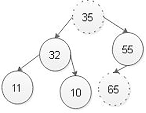
When searching, the node we would like to search for is called a key node. The key node will be matched with each node starting from the root node if the value of a key node is greater than the current node, then we search for it on the right sub-tree otherwise on the left sub-tree. If we reach the leaf node and still we do not get the value of the key node, then we declare that “node is not present in the binary search tree” (Figure 5.40).

FIGURE 5.40 Binary search tree.

If we want to search node 33, then first compare key node 33 with root 55. Here, 33 < 55, then search the value in the left sub-tree. Now compare 33 with 15, here 33 > 15 so search key node 33 in the right sub-tree. Then compare key node 33 with the right side node of 15, that is, 33, which means 33 = 33, that is, key node 33 can be searched. Then give the message that key node 33 is found in the BST.

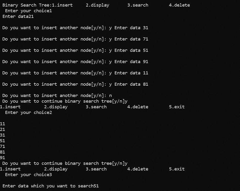
Program: Implementation of BST and perform insertion, deletion, searching, display operations on BST.

#include<stdio.h>
#include<stdlib.h>
struct bst
{
struct bst *left;
int data;
struct bst *right;
};
//Function prototypes
void insert(struct bst * root , struct bst * new1);
void in-order(struct bst *);
struct bst * search(struct bst * root, int key, struct bst **
parent);
void delet(struct bst *, int key);
//main function definition
int main()
{
int choice, key;
char ch;
struct bst *root,*new1,*temp,*parent;
root=NULL;
parent=NULL;
printf("\n Binary Search Tree:");
do
{
printf("1.insert\t 2.display \t 3.search \t 4.delete \t 5.exit
\n ");
printf(" Enter your choice");
scanf("%d", &choice);
switch(choice)
{
case 1:       
do
{
new1=(struct bst *)malloc(sizeof(struct bst));
printf(" Enter data");
scanf("%d",&new1->data);
new1->left=NULL;
new1->right=NULL;
if(root==NULL)
{
root=new1;
}
else
{
insert(root,new1);
}
printf("\n Do you want to insert another node[y/n]: ");
ch=getche();
}while(ch=='y'|| ch=='Y');
break;
case 2:
if(root==NULL)
printf("\n First create Binary Search Tree");
else
in-order(root);
break;
case 3:
if(root==NULL)
printf("\n First create Binary Search Tree");
else
{
printf("\n Enter data which you want to search");
scanf("%d", &key);
temp=search(root, key, &parent);
printf("\n%d", temp->data);
}
break;
case 4:
if(root==NULL)
printf("\n First create Binary Search Tree ");
else
{
printf("\n Enter data which you want to delete");
scanf("%d", &key);
delet(root, key);
}
break;
case 5:
exit(0);
default:
printf("\n Wrong choice");
}
printf("\n Do you want to continue binary search tree[y/n]");
fflush(stdin);
scanf("%c",&ch);
}while(ch=='y' || ch=='Y');
return 0;
}
//insert an element in a binary search tree
void insert(struct bst *root, struct bst *new1)
{
if(root->data<new1->data)
{
        if(root->right==NULL)
        {
        root->right=new1;
        }
        else
        {
        insert(root->right, new1);
        }
}
if(root->data>new1->data)
{
        if(root->left==NULL)
        {
        root->left=new1;
        }
        else
        {
        insert(root->left, new1);
        }
}
}
//search a node in a binary search tree and return address of
searched node and address of its //parent node
struct bst * search(struct bst *root, int key, struct bst
**parent)
{
struct bst *temp;
temp=root;
while(temp!=NULL)
{
        if(temp->data==key)
        {
        printf("\n Node is found");
        return temp;
        }
        else
        {
        *parent=temp;   //update address of parent node in
        calling function also
        if(temp->data<key)
        {
        temp=temp->right;
        }
        else
        {
        temp=temp->left;
        }
        }   // completion of outer else statement
} //completion of while loop
   
printf("\n Node is  not found");  
return NULL;   //if node is not present in binary search tree
then return NULL address
}  // completion of search function
//delete a node from binary search tree
void delet(struct bst *root, int key)
{
struct bst * parent, *temp, *temp_succ;
temp =search(root, key, &parent);
if(temp == NULL)
{
printf("\n Node is not found in Binary search tree");
return ;
}
if(temp == root)
{
printf("\n Node which you want to delete is the root node and
we cannot delete root");
return ;
}

//deleting a node having two children 
if( (temp->right!=NULL) && (temp->left!=NULL) )
{
parent=temp;
temp_succ=temp->right;
while(temp_succ->left!=NULL)   //find in-order successor of
temp node
{
parent=temp_succ;
temp_succ=temp_succ->left;
}
temp->data=temp_succ->data;  //copy data of in-order successor
node data into temp node
if(temp_succ==temp->right)    //if in-order successor node is
right side of temp node
{
parent->right=NULL;
}
else      //if in-order successor node is left side of temp
node
{
parent->left=NULL;
}
free(temp_succ);     //free in-order successor node 
temp_succ = NULL;
}
//deleting a node having only right child 
else if((temp->right!=NULL)&&(temp->left==NULL))
{
if(parent->right==temp)   //find whether temp node is left or
right side of parent node
{
parent->right=temp->right;
}
else
{
parent->left=temp->right;
}
temp->right=NULL;
temp->left=NULL;
free(temp);
temp=NULL;
}
//deleting a node having only left child 
else if((temp->right==NULL)&&(temp->left!=NULL))
{ 
if(parent->left==temp)  //find whether temp node is left or
right side of parent node
{
parent->left=temp->left;
}
else
{
parent->right=temp->left;
}
temp->right=NULL;
temp->left=NULL;
free(temp);
temp=NULL;
}
//deleting a node having no child that is leaf node 
else if((temp->right==NULL)&&(temp->left==NULL))
{
if(parent->left==temp)  //find whether temp node is left or
right side of parent node
{
parent->left=NULL;
}
else
{
parent->right=NULL;
}
free(temp);
temp=NULL;
}
printf("\n Deleted node in BST = %d", key);
}
//display binary search tree in in-order traversing method
void in-order(struct bst *temp)
{
if(temp!=NULL)
{
in-order(temp->left);
printf("\n%d",temp->data);
in-order(temp->right);
}
}

Output:

5.6 BST Algorithms

1. Create BST algorithm:
2. Insert new node in a BST algorithm:
3. Search node in a BST algorithm:
4. Delete any node from a BST algorithm:
5. In-order traversing in a BST algorithm:

5.6.1 Create BST Algorithm

Step 1: Start

Step 2: First, create a structure for the BST node as follows:

struct bst
{
struct bst *left;   //Store address of left sub-tree
int data;               // Store the data in a node
struct bst *right; // Store address of right sub-tree
};

Step 3: Initialize the structure’s pointer type of variables such as root, parent, new1 and temp as a NULL.

Step 4: Create a new node using dynamic memory management as

new1=( struct bst * )malloc (sizeof (struct bst) );

Here, malloc() function reserves the block of memory required for the new node and that address is stored into the new1 pointer type of variable.

Step 5: Then insert new data into the data part of the newly created node also make right and left pointer as NULL using,

printf("Enter data into new node");
scanf("%d", &new1->data);
new1->left=NULL;
new1->right=NULL;

Step 6: Check whether or not the root node has a NULL address. If the root contains a NULL address, then assign the address of the new node to the root.

Step 7: Otherwise, if the root node contains some address other than NULL, then, call to insert function and pass root node’s address and newly created node’s address as an argument.

Step 8: Ask the user to insert more nodes in the BST.

Step 9: If the user said yes, then repeat steps 4–8.

Step 10: If the user said no, then stop creating BST.

Step 11: Stop

5.6.2 Insert New Node in BST Algorithm

Algorithm insert(struct bst *root, struct bst *new1)

Step 1: Start

Step 2: Check the data in the root node and in the new node. If the root node’s data are less than the new node’s data, then go to the right sub-tree. In addition, check whether or not the root node’s right pointer contains the NULL address. If the root node’s right pointer contains the NULL address, then attach a new node to the current root node’s right. Otherwise, call the insert function recursively with the new root node’s address and address of the newly created node. Here, the current root node contains the address of the right sub-tree. Here, the address of newly created node’s address remains the same, which is shown as follows:

if(root->data < new1->data)
{
      if(root->right==NULL)
      {
      root->right=new1;
      }
      else
      {
      insert(root->right, new1);
      }
}

Step 3: Check the data in the root node and in the new node. If the root node’s data is greater than the new node’s data, then go to the left sub-tree. In addition, check whether the root node’s left pointer contains the NULL address or not. If the root node’s left pointer contains the NULL address, then attach a new node to the current root node’s left. Otherwise, call the insert function recursively with the new root node’s address and address of the newly created node. Here current root node contains the address of the left sub-tree. Here, the address of newly created node’s address remains the same, which is shown as follows:

if(root->data > new1->data)
{
      if(root->left==NULL)
      {
      root->left=new1;
      }
      else
      {
      insert(root->left, new1);
      }
}

Step 4: If the new node is placed in its correct position, then stop calling the insert function recursively.

Step 5: Stop

5.6.3 Search Node in BST Algorithm

Algorithm struct bst * search (struct bst *root, int key, struct bst **parent)

Step 1: Start

Step 2: Check whether a BST is created or not.

If root=NULL, then

Print “ First create Binary Search Tree.”

Otherwise

Take the key from the user whom you want to search in a BST.

Step 3: Copy address of root node in temp pointer for traversing purpose.

temp= root

Step 4: Check the temp pointer’s data part with the key, which you want to search till the temp pointer contains the NULL address. If temp pointer’s data and key are matched, then display the message “Node is found” and return the address of the searched node.

Step 5: If temp pointer’s data and key are not matched, then copy the address of current temp into parent pointer as follows:

*parent=temp;

Step 6: If temp pointer’s data are less than the key value, then assign the address of the right sub-tree to the temp pointer.

if (temp->data<key)
{
temp=temp->right;
}

Step 7: Otherwise assign the address of the left sub-tree to the temp pointer.

temp=temp->left;

Repeat steps 4–7 till the temp pointer contains a NULL address.

Step 8: If the temp pointer contains the NULL address, then print “Node is not found."

Step 9: Stop.

5.6.4 Delete Any Node from BST Algorithm

Algorithm delet (struct bst *root, int key)

Step 1: Start

Step 2: Check whether or not a BST is created.

If root=NULL, then

Print “First create Binary Search Tree."

Otherwise

Take the key from the user whom you want to delete from the BST.

Step 3: Call to search function. After the execution of the search function returns two addresses, one address of node that we want to delete in temp pointer and another address of parent node which we want to delete into parent pointer.

Step 4: First check whether or not the temp pointer is NULL. If the temp pointer is NULL, then print the message “Node is not found in Binary search tree” and return to the calling function.

Step 5: If the temp pointer is not NULL, then check whether a temp pointer contains the address of the root node. If temp contains the address of root node, then print message “Node which you want to delete is a root node and we cannot delete root” and return to the calling function.

Step 6: If temp pointer does not contain addresses of the root node, then check node that we want to delete having two children, if this condition is true, then found its in-order successor and replace the deleted node value by in-order successor node’s value and free the in-order successor node from the BST.

                        if( (temp->right!=NULL) && (temp->left!=NULL) )
                        {
                        parent=temp;
                        temp_succ=temp->right;
                        while(temp_succ->left!=NULL)   //find in-order successor of
                        temp node
                        {
                        parent=temp_succ;
                        temp_succ=temp_succ->left;
                        }
                        temp->data=temp_succ->data;  //copy data of in-order
                        successor node data into temp 
                             //node
                        if(temp_succ==temp->right)    //if in-order successor
                        node is right side of temp node
                        {
                        parent->right=NULL;
                        }
                        else      //if in-ordersuccessor node is left side of temp node
                        {
                        parent->left=NULL;
                        }
                        free(temp_succ);     //free in-order successor node 
                        temp_succ = NULL;
                        }

Step 7: If the node that we want to delete does not contain two children, then check whether the node contains the right child only. If this condition is true, then find whether the temp node is the left or right side of the parent node. If the temp node is the right side of the parent node, then assign the address of the temp node’s right pointer address to the parent node’s right pointer address. Otherwise, assign the address of the temp node’s right pointer address to the parent node’s left pointer address. In addition, free the temp node.

                        else if((temp->right!=NULL)&&(temp->left==NULL))
                        {
                        if(parent->right==temp)   //find whether temp node is
                        left or right side of parent node
                        {
                        parent->right=temp->right;
                        }
                        else
                        {
                        parent->left=temp->right;
                        }
                        temp->right=NULL;
                        temp->left=NULL;
                        free(temp);
                        temp=NULL;
                        }

Step 8: If the node that we want to delete does not contain only the right child, then check whether the node contains the left child only. If this condition is true, then find whether the temp node is the left or right side of the parent node. If the temp node is the right side of the parent node, then assign the address of the temp node’s left pointer address to the parent node’s right pointer address. Otherwise, assign the address of the temp node’s left pointer address to the parent node’s left pointer address. In addition, free the temp node.

                        else if((temp->right==NULL)&&(temp->left!=NULL))
                        { 
                        if(parent->left==temp)  //find whether temp node is left
                        or right side of parent node
                        {
                        parent->left=temp->left;
                        }
                        else
                        {
                        parent->right=temp->left;
                        }
                        temp->right=NULL;
                        temp->left=NULL;
                        free(temp);
                        temp=NULL;
                        }

Step 9: If the node that we want to delete does not contain only the left child, then check whether the node does not contain both left and right child. If this condition is true, then find whether the temp node is the left or right side of the parent node. If the temp node is the left side of the parent node, then the parent node’s left pointer is assigned address as NULL, otherwise the parent node’s right pointer is assigned address as NULL. In addition, free the temp node.

                        else if((temp->right==NULL)&&(temp->left==NULL))
                        {
                        if(parent->left==temp)  //find whether temp node is left
                        or right side of parent node
                        {
                        parent->left=NULL;
                        }
                        else
                        {
                        parent->right=NULL;
                        }
                        free(temp);
                        temp=NULL;
                        }

Step 10: After checking all conditions, the print value of the deleted node.

Step 11: Stop

                        //display binary search tree in in-order traversing
                        method
                        void in-order(struct bst *temp)
                        {
                        if(temp!=NULL)
                        {
                        in-order(temp->left);
                        printf("\n%d",temp->data);
                        in-order(temp->right);
                        }
                        }

5.6.5 In-order Traversing of BST Algorithm

In-order traversing of the BST T with root R.

Algorithm in-order (root R)

1. Traverse the left sub-tree of root R, that is, call in-order (left sub-tree)
2. Visit the root, R and process.
3. Traverse the right sub-tree of root R, that is, call in-order (right sub-tree)

5.7 Applications of Binary Tree and BST

1. BST is used to implement dictionary.
2. BST is used to implement multilevel indexing in the database.
3. BST is used to implement the searching algorithm.
4. Heaps is a special type of binary tree: Used in implementing efficient priority queues, which in turn are used for scheduling processes in many operating systems, quality-of-service in routers and the path-finding algorithm used in artificial intelligence applications, including robotics and video games. It is also used in heap-sort.
5. Syntax tree: In the syntax analysis phase of the compiler, parse tree or syntax tree is drawn for parsing expressions either top-down parsing or bottom-up parsing.
6. BST is used in Unix kernels for managing a set of virtual memory areas (VMAs). Each VMA represents a section of memory in a Unix process.
7. Each IP packet sent by an Internet host is stamped with a 16-bit id that must be unique for that source-destination pair. The Linux kernel uses an AVL tree or height-balanced tree for an indexed IP address.
8. BST is used to efficiently store data in a sorted form in order to access and search stored elements quickly.
9. BST is used in dynamic sorting.
10. Huffman Code Construction: A method for the construction of minimum redundancy codes. Huffman code is a type of optimal prefix code that is commonly used for lossless data compression. The algorithm has been developed by David A. Huffman. The technique works by creating a binary tree of nodes. The nodes count depends on the number of symbols.

The main idea is to transform plain input into variable-length code. As in other entropy encoding methods, most common symbols are generally represented using fewer bits than less common symbols.

Huffman Encoding:

A type of variable-length encoding that is based on the actual character frequencies in a given document.

Huffman encoding uses a binary tree:

1. To determine the encoding of each character.
2. To decode an encoded file that is to decompress a compressed file, putting it back into ASCII. Example of a Huffman tree for a text with only six characters:

Leaf nodes are characters.

Left branches are labeled with a 0, and right branches are labeled with a 1.

If you follow a path from root to leaf, you get the encoding of the character in the leaf.

Example: 101 = ‘j’ and 01 = ‘m’.

Characters that appear more frequently are nearer to the root node, and thus their encodings are shorter and require less memory.

Building Huffman tree:

1. First reading through the text, determine the frequencies of each character.
2. Create a list of nodes with character and frequency pairs for each character within the text sorted by frequency.
3. Remove and combining the nodes with the two minimum frequencies, creating a new node that is their parent.
   1. – The left child with the lowest frequency node.
   2. – The right child with the second lowest frequency node.
   3. – The frequency of the parent node has the sum of the frequencies of its children, which is the left and right child.
4. Add the parent to the list of nodes maintaining the sorted order of the list.
5. Repeat steps 3 and 4 as long as there is only a single node in the list, which will be the root of the Huffman tree indicated in Figure 5.41.

   

   FIGURE 5.41 Huffman tree.

11. Binary trees are a good means of expressing arithmetical expressions. The leaves or exterior nodes are operands, and the interior nodes are operators. Two usual types of expressions that a binary expression tree can describe are algebraic and Boolean. These binary trees can represent expressions that incorporate both unary and binary operators.

Each node of a binary tree, that is, in a binary expression tree, has zero, one, or two children. This constricted arrangement simplifies the processing of expression trees.

5.8 Heaps

5.8.1 Basic of Heap data Structure

The heap data structure is a special type of binary tree.

Binary heap is of two types:

1. Max heap
2. Min heap

5.8.2 Definition of Max Heap

Max heap is defined as follows:

A heap of size ‘n’ is a binary tree of ‘n’ nodes that satisfies the following two constraints:

1. The binary tree is an almost complete binary tree. That is, each leaf node in the tree is either at level d or at level d-1, which means that only one difference between levels of leaf nodes is permitted. At depth d, that is the last level, if a node is present, then all the nodes to the left of that node should also be present first and no gap between the two nodes from left to the right side of level d.
2. Keys in nodes are arranged such that the content or value of each node is less than or equal to the content of its father or parent node, which means for each node info[i] <= info[j], where j is the father of node i. This heap is called as max heap.

Here, in heap, each level of binary tree is filled from left to right, and a new node is not placed on a new level until the preceding level is full.

In a min binary heap, the key at the root must be minimum among all keys present in Binary Heap. The same characteristic must be iteratively true for all nodes in a binary tree.

Examples of Max Heap (Figure 5.42).

FIGURE 5.42 Examples of max heap and not max heap.

5.8.3 Operations Performed on Max Heap

The following operations are performed on a max heap data structure:

1. Insertion or creation of heap
2. Deletion
3. Finding a maximum value.

5.8.3.1 Insertion Operation in Max Heap

Insertion operation in max heap is carried out using the following algorithm:

Step 1: Start

Step 2: Add the new node as the last leaf from left to right.

Step 3: Check the new node value against its parent node.

Step 4: If the new node value is greater than its parent, then swap both of them.

Step 5: Repeat steps 3 and 4 as long as the new node value is lesser than its parent node or the new node reaches the root.

Step 6: Stop

Inserting a new key takes O (log n) time.

Example (Figure 5.43):

FIGURE 5.43 Max heap of size 5.

The above binary tree is an almost complete binary tree and the content or value of each node is lesser than the content of its father or parent node and each level of binary tree is filled from left to right, that is, binary tree satisfying both ordering property and structural property according to the max heap data structure so above binary tree is max heap of size 5.

Now insert a new node with a value 65 in above max heap of size 5.

Step 1: Insert the new node with value 65 as a last leaf from left to right, which means the new node is added as a left child of the node with value 35. After adding 65, max heap is as follows:

Step 2: Compare the new node value (65)withitsparent node value (35). That means65 > 35

Here the new node value (65) is greater than its parent value (35), then swap both of them. After sapping, max heap is as shown in below figure:

Step 3: Now, again compare a new node value (65) with its parent node value (55). Here the new node value (65) is greater than its parent value (55), then swap both of them. After sapping, max heap is as shown in below figure:

Step 4: Now new node is a root node hence stopping comparing and the final heap of size 6 is as shown in the Figure 5.44.

FIGURE 5.44 Max heap of size 6 after insertion of node 65.

5.8.3.2 Deletion Operation in Max Heap

In a max heap, removing the last node is very straightforward as it does not disturb max heap characteristics. Removing a root node from a max heap is challenging as it disturbs the max heap characteristics. We use the below steps to remove the root node from the max heap.

Step 1: Start

Step 2: Interchange the root node with the last node in max heap.

Step 3: After interchanging, remove the last node.

Step 4: Compare the root node value with its left child node value.

Step 5: If the root value is smaller than its left child, then compare the left child node value to its right sibling. If not, continue with step 7.

Step 6: If the left child value is larger than its right sibling, then interchange root with the left child. Otherwise, swap root with its right child.

Step 7: If the root value is larger than its left child, then compare the root value with its right child value.

Step 8: If the root value is smaller than its right child, then swap root with the right child. Otherwise, stop the process.

Step 9: Repeat the same one until the root node is set to the correct position.

Step 10: Stop.

Inserting a key takes O (log n) time.

Example (Figure 5.45):

FIGURE 5.45 Max heap of size 6.

In the above max heap, if we want to delete 65 root nodes, then follow the following steps:

Step 1: Swaptheroot node 65withthelast node 35in max heap. After swapping, the max heap is as follows:

Step 2: Delete the last node that is 65 from max heap. After deleting node with value 65 from max heap, the max heap is as follows:

Step 3: Compare root node 35 with its left child 32. Here, the node with value 35 is larger than its left child. Therefore, we compare node with value 35 is compared with its right child 55. Here, the node with value 35 is smaller than its right child 55. Therefore, we swap both of them. After swapping, max heap is as follows:

Here, the node with value 35 does not have left and right child. Therefore, we stop the process.

Finally, max heap after deleting root node 65 is as follows:

5.8.3.3 Finding Maximum Value in Max Heap

Finding the node with the maximum value in a max heap is quite simple. In max heap, the root node has the maximum value as all other nodes in the max heap. Thus, directly we can display the value of the root node as the maximum value in the max heap.

5.8.4 Applications of Heaps

1. Heap Sort: Heap sort uses a binary heap for sorting an array in O (n log n) time.
2. Graph Algorithms: The priority queues are particularly used in graph algorithms like Dijkstra’s shortest path and Prim’s minimum spanning tree.
3. Priority Queue: Priority queues may be implemented effectively using binary heap.
4. Many problems can be resolved effectively by utilizing heaps such as:
   1. Nth largest element in an array.
   2. Sort an almost sorted array.
   3. Merge N number of sorted arrays.

5.9 AVL Tree

5.9.1 Introduction of AVL Tree

The AVL tree is a self-balanced BST. That means, an AVL tree is also a BST, but it is a balanced tree. A binary tree is said to be balanced, if the difference between the heights of the left sub-trees and right sub-trees of every node in the tree is either −1, 0 or +1. In other words, a binary tree is said to be balanced if for every node’s height of its children differs by at most one. In an AVL tree, every node maintains extra information known as balance factor. The AVL tree was initiated in the year 1962 by G.M. Ade’son-Ve’skii and E.M. Landis in their honor’s height balanced BST is termed as AVL tree. In the complete balanced tree, left and right sub-trees of any node would have the same height. Every AVL Tree is a BST, but all the BSTs need not to be AVL trees.

5.9.2 Definition

An empty tree is height-balanced, if T is a non-empty BST with T_L and T_R as its left and right sub-tree, then T is height-balanced if,

1. T_L and T_R are height-balanced and
2. | h_L - h_R | <= 1.

where h_L and h_R are the heights of T_L and T_R, respectively.

An AVL tree is a balanced BST. In an AVL tree, the balance factor of every node is either −1, 0 or +1.

The balance factor of a node is the difference between the heights of the left and right sub-trees of that node. The height of the left sub-tree – height of the right sub-tree or height of the right sub-tree – height of the left sub-tree is used to compute the balancing factor of a node. In the following explanation, we calculate as follows:

Balance factor (T) = height of left sub-tree – height of right sub-tree

where T is a binary tree.

BF (T) = −1, 0, 1.

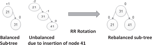
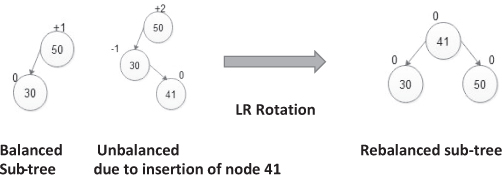
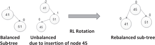
If AVL tree’s balance factor is exceeding the value 1 for any of the nodes, then rebalancing has to be taken place. After each insertion and deletion of items, if the balance factor of any node exceeds value 1, then rebalancing of the tree is carried out by using different rotations. These rotations are characterized by the nearest ancestor of the newly inserted node whose balance factor becomes +2 or −2.

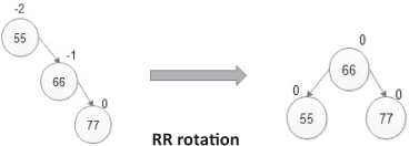
5.9.3 AVL Tree Rotations

In the AVL tree, after each operation such as inserting and deleting, we have to check the balance factor of each node in the tree. If each node fulfills the balance factor condition, then we conclude the operation; otherwise, we must make it balanced. We use rotation operations to balance the tree every time the tree becomes unbalanced because of any operation.

Rotation operations are used to balance a tree.

Rotation is the movement of the nodes to the left or right to balance the tree.

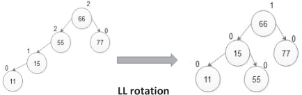
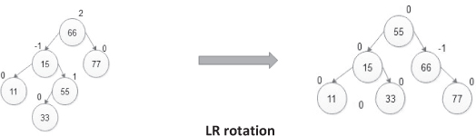
The following are four types of rotations:

1. 1. L L rotation
2. 2. R R rotation
3. 3. L R rotation
4. 4. R L rotation

Example:

1. L L rotation:

   It is used when a new node is inserted in the left sub-tree of the left sub-tree of node A.

   
2. R R rotation:

   It is used when a new node is inserted in the right sub-tree of the right sub-tree of node A.

   
3. L R rotation:

   It is used when a new node is inserted in the right sub-tree of the left sub-tree of node A.

   
4. R L rotation:

   It is used when a new node is inserted in the left sub-tree of the right sub-tree of node A.

   

5.9.4 Operations on an AVL Tree

The following operations are carried out in an AVL tree:

1. Search a node in an AVL tree
2. Insertion of a node in an AVL tree
3. Deletion of a node from an AVL tree.

5.9.4.1 Search Operation in AVL Tree

In the AVL tree, the search operation is executed with a time complexity O (log n). The search operation is conducted in the same way as the search operation of the BST. We use the subsequent steps to search an element in an AVL tree:

1. Step 1: Start
2. Step 2: Read the search element from the user.
3. Step 3: Next, compare the search element to the root node value in the tree.
4. Step 4: If both are equal, then display “Element is Searched” and wind up the search function.
5. Step 5: If both are not equal, then verify whether a search element is smaller or greater than that of the parent node value.
6. Step 6: If the search element is smaller, then continue the search process in the left sub-tree.
7. Step 7: If the search element is larger, then continue the search process in the right sub-tree.
8. Step 8: Repeat the same as long as we find the exact element or we finish with a leaf node.
9. Step 9: If we reach the node with a search value, then display “Element is Searched” and terminate the function.
10. Step 10: If we reach a leaf node and it is also not matching, then display “Element is not Searched” and terminate the function.
11. Step 11: Stop.

5.9.4.2 Insertion Operation in AVL Tree

In the AVL tree, the insertion activity is carried out with O (log n) time complexity. In the AVL Tree, the new node is always inserted as a leaf node. The insertion operation is carried out as follows:

1. Step 1: Start
2. Step 2: Insert the new item in the tree with the BST insertion logic.
3. Step 3: Once inserted, check the balance factor for each node.
4. Step 4: If the balance factor of every node is 0 or 1 or −1, then go to step 6.
5. Step 5: If the balance factor of a node is not 0 or 1 or −1, then the tree is said to be unbalanced. Then perform the appropriate rotation technique to achieve balance. In addition, get on with the next operation.
6. Step 6: Stop.

Example:

Insertion of the following nodes in an AVL tree:

55, 66, 77, 15, 11 and 33

New Identifier	After Insertion	Rotation Technique	After Rebalancing
55			No rebalancing needed
66			No rebalancing needed
77
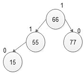
15			No rebalancing needed
11
33

5.9.4.3 Deletion Operation in AVL Tree

In the AVL Tree, the deletion operation is similar to the deletion operation in BST. However, after each deletion operation, we must necessary to check with the balance factor condition. If the tree is balanced after deletion, then go to the next operation otherwise perform the proper rotation to make the tree balanced.

5.9.5 Advantages

1. When compared to the number of insertion and deletions, the number of times a search operation is carried out is relatively large. The use of an AVL tree always results in superior performance.
2. The main objective here is to keep the tree balanced at all times. Such balancing causes the depth of the tree to remain at its minimum, reducing the overall cost of search.
3. AVL tree gives the best performance for dynamic tables.

5.9.6 Disadvantages

1. Insertion and deletion of any node from an AVL tree become complicated.

5.10 B Trees

5.10.1 Introduction of B Tree

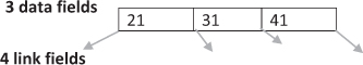
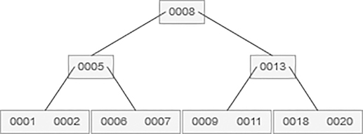
B tree is not a binary tree. B tree is a balanced m-way tree that is each tree node contains a maximum of (m-1) data elements in the node and has m branches or links.

For example, a balanced four-way tree node contains three data fields and four-link fields shown as follows:

B tree finds its use in external sorting.

In a BST, AVL Tree, every node can have only one value or key and a maximum of two children, but there is some other type of search tree called B-Tree in which a node can store more than one value or key and it can have more than two children. B-Tree was developed in 1972 by Bayer and McCreight with the name Height Balanced m-way Search Tree. Later, it was termed as B-Tree.

B-Tree can be defined as follows:

1. The B-Tree is a self-balanced search tree with multiple keys in every node and more than two children for every node. In this case, the number of keys in a node and the number of children for a node depend on the order of the B-Tree. Every B-Tree has an order.

5.10.2 B-Tree of Order m Has the Following Properties

1. All the leaf nodes must be at the same level.
2. Each node has a maximum of m children.
3. Each node has one fever key than children with a maximum of m-1 keys or data values.
4. The keys are arranged in defining order within a node such as ascending order. In addition, all keys in the left sub-tree are less valuable than key and the right sub-tree has greater value.
5. 5. When a new key is to be inserted into a full node, the node is split into two nodes and key with a median value is inserted into the parent node. If the parent node is root and it is likewise full, then a new root is created.

For example, B-Tree of Order 4 contains maximum three key values in a node and maximum four children for a node.

5.10.3 Operations on a B-Tree

1. B-Tree Insertion:
2. B-Tree Deletion:
3. Search Operation in B-Tree:

5.10.3.1 B-Tree Insertion

In a B-Tree, the new element should only be added to the leaf nodes. This means that the new value of the key remains attached to the leaf node only. The insertion operation takes place as follows:

1. Step 1: Start
2. Step 2: First verify if the tree is empty.
3. Step 3: If the tree is empty, create a new node with a new key value and place it in the tree as the root node.
4. Step 4: If the tree is not empty, then discover a leaf node to which the new key value can be inserted using the BST logic.
5. Step 5: If that leaf node has an empty place, then add the new key value for that leaf node by preserving ascending order of the key value as part of the node.
6. Step 6: If that leaf node is already full, then split that leaf node by sending a middle value to its parent node. Repeat the same until sending value is fixed into a node.
7. Step 7: If the splitting has taken place of the root node, then the middle value becomes a new root node in the tree, and the height of the tree is increased by one.
8. Step 8: Stop.

Example:

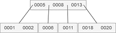
Consider a building of B-tree of order or degree 4 that is a balanced four-way tree where each node can hold three data values and have four links or branches.

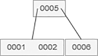
Suppose we want to insert the following data values in B-tree, 1, 5, 6, 2, 8, 11, 13, 18, 20, 7, 9.

Steps:

First, value 1 is placed in a node, which can also accommodate next two values, that is, 5 and 6.

When the fourth value 2 is to be added, the node is split at a median value 5 into leaf nodes with a parent at 5.

Then, 8 and 11 are added to a leaf node.

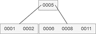
13 is to be added. However, the right leaf node is full. Therefore, it is split at a median value 8 and thus 8 moves up to the parent. In addition, the right leaf node is split into nodes.

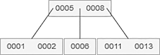
18 is to be added, which is shown as follows:

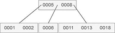
20 is to be added, which is shown as follows:

Next 7 and then 9 is to be added, which is shown as follows:

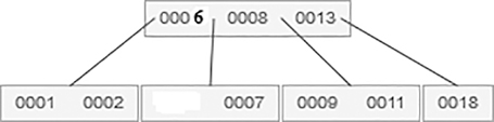
5.10.3.2 B-Tree Deletion

The delete method lets you search for the first record you want to delete.

1. If the record is in the terminal node, the deletion is straightforward. The record along with the appropriate pointer is deleted.
2. If the record is not in the terminal node, it is replaced by a copy of its successor, which is a record with a higher subsequent value.

Example:

If 20 is searched, then delete 20 from that node. After the deletion, B-tree is like as follows:

If element 5 is deleted, then find its successor node element that is 6 and replace 5 with 6.

After deletion of element 5, B-tree becomes as follows:

5.10.3.3 Search Operation in B-Tree

In a B-tree, the search function is the same as that of BST. In a BST, the search process begins from the root node and the rest of time we make a two-way decision either we go to the left sub-tree or we go to the right sub-tree. In a B-Tree, the search process starts from the root node, but every time we make an n-way decision where n is the total number of children that node has. In a B-tree, the search operation is performed with O (log n) time complexity. The search procedure is carried out as follows:

1. Step 1: Start.
2. Step 2: First, read the search element from the end user.
3. Step 3: Then compare, the search element with the first key value of the root node in the tree.
4. Step 4: If both are equal, then display “Given node is searched” and wind up the function.
5. Step 5: If both are not matching, then verify whether a search element is smaller or larger than that key value.
6. Step 6: If the search element is smaller, then continue the search process in the left sub-tree.
7. Step 7: If the search element is larger, then compare with the next key value in the same node and repeat steps 3, 4, 5 and 6 until we found an exact match or comparison completed with the last key value in a leaf node.
8. Step 8: If we completed with last key value in a leaf node, then display “Element is not found” and terminate the function.
9. Step 9: Stop.

5.10.4 Uses of B-tree

1. External sorting purpose B-tree is used.
2. B tree is used in a database management system.

5.11 B+ Trees

5.11.1 Introduction of B+ Tree

B+ tree is not a binary tree. B+ tree is a balanced m-way tree, that is, each tree node contains a maximum of (m-1) data elements in the node and have m branches or links.

In B+ tree, all leaves have been joined to form a linked list of keys in a sequential order.

B+ tree has two parts:

1. The index part is interior nodes.
2. The sequence set is the leaves or exterior nodes.

The linked leaves are a brilliant aspect of B+ tree. Keys can be accessed effectively both directly and sequentially. B+ tree is used to offer indexed sequential file organization. The key values in the sequence set are the key values in the record collection. The key values in the index part exist solely for internal purposes of direct access to the sequence set.

In the B+ tree, + indicates extra functionality than that of the B-tree, that is, leaf nodes are connected.

5.11.2 B+ Tree of Order m Has the Following Properties

1. All the leaf nodes must be at the same level.
2. Each node has a maximum of m children or link parts.
3. Each node has one fever key than children with a maximum of m-1 keys or data values.
4. The keys are arranged in a defining order within a node such as ascending order. In addition, all keys in the left sub-tree are less value than key and the right sub-tree has a greater value.
5. When a new key is to be inserted into a full node, the node is split into two nodes, and key with a median value is inserted into the parent node. If the parent node is root and it is likewise full, then a new root is created.
6. All leaves have been connected to form a linked list of keys in sequential order.

For example, the B+ Tree of order 3 contains maximum two key values in a node and maximum three children or link part of a node.

5.11.3 Operations on a B+ Tree

1. B+ Tree Insertion:
2. B+ Tree Deletion:
3. Search Operation in B+ Tree:

5.11.3.1 B+ Tree Insertion

B+ tree insertion algorithm:

In a B+ Tree, the new element must be added only at leaf nodes. That means, always the new key value is attached to the leaf node only. The insertion operation is performed as follows:

1. Step 1: Start.
2. Step 2: First verify if the tree is empty.
3. Step 3: If the tree is empty, create a new node with a new key value and place it in the tree as the root node.
4. Step 4: If the tree is not empty, then discover a leaf node to which the new key value can be added using BST logic.
5. Step 5: If that leaf node has an empty position, then add the new key value for that leaf node by preserving ascending order of key value within the node.
6. Step 6: If that leaf node is already full, then split that leaf node by sending the median value to its parent node. Repeat the same until sending value is fixed into a node.
7. Step 7: If the splitting is occurring to the root node, then the median value becomes a new root node in the tree and the height of the tree is increased by one.
8. Step 8: After inserting a new key value into B+ tree, all leaves have been connected to form a linked list of keys in sequential order.
9. Step 9: Stop.

Example:

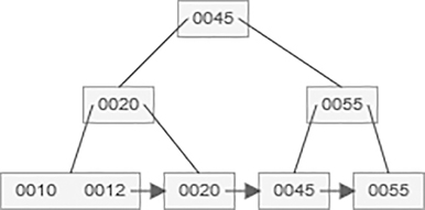
Consider a building of the B+ tree of order or degree 3 that is a balanced three-way tree where each node can hold two data values and have three links or branches.

Suppose we want to insert the following data values in the B+-tree, 10, 20, 30, 12, 21, 55 and 45.

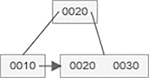
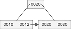
Here, the B+ tree of order 3 having two data part. Therefore, we first insert 10 in a node then 20 data at the next right empty field in node, then B+ tree looks like as follows:

After the insertion of values 30 in the B+ tree node, split, then node having median 20 and make that node as a parent node and insert 20 and 30 value into one node and 10 values in another node and now these two nodes become leaf nodes, so connect that two nodes using a linked list. After inserting value 30, B+ tree looks like as follows:

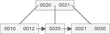
After insertion of 12 value in B+ tree,

After insertion of 21 value in B+ tree,

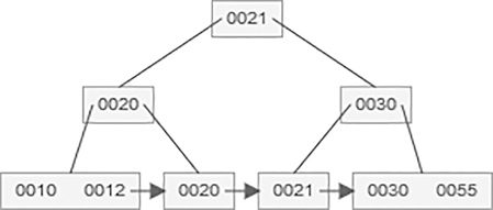
After insertion of 55 value in B+ tree,

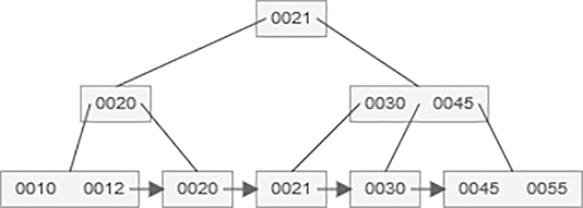
After insertion of 45 value in B+ tree,

5.11.3.2 B+ Tree Deletion

B+ tree deletion algorithm:

1. If the deleted key is the indexed node’s value, then delete the index node’s key and data from the leaf node.
2. If the leaf node underflows, merge with siblings and delete key in between them.
3. If the index node underflows, merge with siblings and move down key in between them.

Deletion of 30 values from above B+ tree, then 30 values are in both leaf node and index node. Therefore, delete the value from both leaf and index node. Then index node goes underflow condition, so the successor key value 55 becomes median and goes to its parent node. Therefore, 45 and 55 values are now present in the parent node, that is, the index node.

Deletion of 21 value from above B+ tree,

5.11.3.3 Search Operation in B+ Tree

In a B+ tree, the search operation is the same as that of BST. In a BST, the search process initiates from the root node, and each time we make a two-way decision: either we go to the left sub-tree or we go to the right sub-tree. In a B+ tree also, the search method starts from the root node, but every time we make an n-way decision where n is the total number of children that node has. In a B-tree, the search operation is carried out with O (log n) time complexity. The search process is carried out as follows:

1. Step 1: Start.
2. Step 2: First, read the search element from the end user.
3. Step 3: Then compare the search element with a first key value of the root node in the tree.
4. Step 4: If both are equal, then display “Given node is found” and terminate the function.
5. Step 5: If both are not matching, then check whether a search element is smaller or larger than that key value.
6. Step 6: If the search element is smaller, then continue the search process in the left sub-tree.
7. Step 7: If the search element is larger, then compare with the next key value in the same node and repeat steps 3, 4, 5 and 6 until we find an exact match or comparison completed with a last key value in a leaf node.
8. Step 8: If we accomplished with last key value in a leaf node, then display “Element is not found” and wind up the function.
9. Step 9: Stop.

5.11.4 Uses of B+ Tree

1. For the external sorting purpose, B+ tree is used.
2. B+ trees are used to provide indexed sequential file organization.
3. B+ tree is used in a database management system.

5.12 Interview Questions

1. What are different binary tree traversal techniques?
2. Implement preorder traversal of binary tree using recursion?
3. Explain the difference between binary tree and BST with an example?
4. What are advantages and disadvantages of BST?
5. What is AVL Tree?
6. Why do we want to use BST?
7. Write algorithm for post-order traversing?
8. How do you insert a new element in a BST?
9. What is the minimum number of nodes that a binary tree can have?
10. Write a note on heaps?
11. Explain different ways of deleting of nodes in the BST.
12. Explain tree terminologies with suitable examples?
13. Explain different types of binary tree representation?
14. Write a note on breadth first traversal and depth first traversal?
15. Explain recursive algorithm for in-order traversal?
16. What are the different operations performed on BSTs?
17. Explain different applications of heaps?
18. 18. What is B tree?
19. What is the difference between B Tree and B+ tree?
20. What are advantages and disadvantages of the AVL tree?
21. Define binary tree. Explain different types of binary trees.

5.13 Multiple Choice Questions

1. Assume that we have numbers between 1 and 1000 in a BST and want to search for the number 363. Which of the below ordering could not be the ordering of the node reviewed?
   1. 2, 252, 401, 398, 330, 344, 397, 363
   2. 924, 220, 911, 244, 898, 258, 362, 363
   3. 925, 202, 911, 240, 912, 245, 258, 363
   4. 2, 399, 387, 219, 266, 382, 381, 278, 363

      Answer: C

2. In a complete binary tree or perfect binary tree, every inner node has exactly two children. If there are 21 leaf nodes or exterior nodes in the tree, how many internal nodes are there in the perfect binary tree?
   1. 19
   2. 20
   3. 22
   4. 18

      Answer: B

      Explanation:

      In a complete binary tree or perfect binary tree having n interior nodes, then there are exactly (n+1) leaf or exterior nodes.

3. Which type of traversal of BST produces the value in ascending sorted order?
   1. Preorder traversal
   2. Post-order traversal
   3. In-order traversal
   4. All of the above

      Answer: C

4. A 2-3 is a type of tree which is having the following properties,
   1. 2-3 tree’s all internal nodes have either two or three children.
   2. 2-3 tree’s all paths from root to leaves have the same length
   3. Then the number of internal nodes of a 2-3 tree having nine leaves could be
      1. 4 or 8
      2. 5 or 9
      3. 6 or 7
      4. 7 or 4

      Answer: D

5. If a node has two children that node we want to delete from a BST, then that deleted node must be replaced by its
   1. In-order successor
   2. In-order predecessor
   3. Post-order successor
   4. Post-order predecessor

      Answer: A

6. A BST is formed from the given sequence 6, 9, 1, 2, 7, 14, 12, 3, 8 and 18. The minimum number of nodes required to be added into this tree to form an extended binary tree is?
   1. 3
   2. 6
   3. 8
   4. 11

      Answer: D

7. In a full binary tree, every internal node has exactly two children. A full binary tree with 2n +1 nodes contains,
   1. 2n leaf nodes
   2. n+1 internal nodes
   3. n+1 exterior nodes
   4. n-1 internal nodes

      Answer: C

8. If n numbers are to be sorted in ascending order in O (n log n) time, which of the following tree can be used
   1. Binary tree
   2. Binary search tree
   3. Max-heap
   4. Min-heap

      Answer: D

9. If n elements are sorted in a balanced BST. What would be the asymptotic complexity to search a key in the tree?
   1. A O(1)
   2. O(logn)
   3. O(n)
   4. O(nlogn)

      Answer: B

10. In which of the following tree, parent node has a key value greater than or equal to the key value of both of its children?
    1. Binary search tree
    2. Threaded binary tree
    3. Complete binary tree
    4. Max-heap

       Answer: D

11. A complete binary tree T has n leaf nodes. The number of nodes of degree 2 in T is
    1. log₂n
    2. n-1
    3. n
    4. 2ⁿ

       Answer: B

12. A BST is generated by inserting in order the following integers: 50, 15, 62, 5, 20, 58, 91, 3, 8, 37, 60 and 24.

    The number of the node in the left sub-tree and right sub-tree of the root, respectively, is

    1. (4, 7)
    2. (7, 4)
    3. (8, 3)
    4. (3, 8)

       Answer: B

13. The number of edges or links from the root node to the deepest leaf is called _________ of the tree.
    1. Height
    2. Depth
    3. Length
    4. Width

       Answer: A

       In a complete binary tree or a proper binary tree or a strictly binary tree if the number of internal nodes is N, then the number of leaves or exterior nodes, E are?

       1. E = 2*N -1
       2. E = N + 1
       3. E = N – 1
       4. E = N – 2N

          Answer: B

14. Which of the following statements is false or true?
    1. A full binary tree or a proper binary tree or a strictly binary tree is a binary tree in which each node other than the leaves has one or two children.
    2. All complete binary trees are strictly binary trees, but all strictly binary trees are not complete binary trees.
       1. Statement 1 is false.
       2. Statement 2 is false.
       3. Statements 1 and 2 both are false.
       4. Statements 1 and 2 both are true.

          Answer: (D)

15. Which type of binary tree produces the value in ascending sorted order when it is traversed?
    1. Binary search tree
    2. Complete binary tree
    3. Strictly binary tree
    4. Almost complete binary tree

       Answer: A

16. Which of the following statements is false or true?
    1. If a tree is dominated by the left child node or right child node, it is said to be a skewed binary tree.
    2. Forest is the disjoint union of trees.
       1. Statement 1 is false
       2. Statement 2 is false
       3. Statements 1 and 2 both are false
       4. Statements 1 and 2 both are true

          Answer: (D)

17. Which of the following statements is false or true?
    1. An AVL tree is also a BST, but it is a balanced tree.
    2. Every AVL Tree is a BST, and all the BSTs are also AVL trees.
       1. Statement 1 is false
       2. Statement 2 is false
       3. Statements 1 and 2 both are false
       4. Statements 1 and 2 both are true

          Answer: (B)

18. Which of the following statements is false or true?
    1. B tree is a binary tree.
    2. B+ tree is used to provide indexed sequential file organization.
       1. Statement 1 is false
       2. Statement 2 is false
       3. Statements 1 and 2 both are false
       4. Statements 1 and 2 both are true

          Answer: (A)

19. Which of the following statements is false or true?
    1. In a B+ tree, the search operation is different than that of BST.
    2. Internal sorting purpose B+ tree is used.
       1. Statement 1 is false
       2. Statement 2 is false
       3. Statements 1 and 2 both are false
       4. Statements 1 and 2 both are true

          Answer: (C)

20. Which of the following statements is false or true with respect to a B+ tree?
    1. In a B+ tree, all the leaf nodes must be at the same level.
    2. In a B+ tree, all leaves have been connected to form a linked list of keys in sequential order.
       1. Statement 1 is false
       2. Statement 2 is false
       3. Statements 1 and 2 both are false
       4. Statements 1 and 2 both are true

          Answer: (C)