The matrix method of solution is particularly effective in solving Hill’s equation in cases when the function F(t) may be represented as a sum of step function in the interval ![]() as shown in Fig. 30.1.
as shown in Fig. 30.1.
Let the function F(t) be composed of m step functions each of length T0 and heights h1,h2, . . . , hm, where
Let the following notation be introduced:
Fig. 30.1
it can be seen by reasoning similar to that used in Sec. 29 that at the end of the fundamental interval T= mT0 the solution is given by
The solution at the end of n intervals when t = nT is given by
The stability of the solution is then determined by (29.20).
This method can be used to study the stability and to obtain the approximate solution of equations of the Hill type by representing the given function F(t) throughout the fundamental interval by a sum of step functions as in the method of mean coefficients.1 To illustrate the general procedure, consider a Hill’s equation of the form
where the function F(t) has the form
in the fundamental interval ![]() and is a periodic function of fundamental period T= 1.
and is a periodic function of fundamental period T= 1.
In order to represent the function F(t) by step functions, divide the fundamental interval T= 1 into ten equal subintervals of length ![]() The average value of F(t) in each subinterval will be taken to be equal to the height of the steps. Thus in the kth interval the representative step function will have the height
The average value of F(t) in each subinterval will be taken to be equal to the height of the steps. Thus in the kth interval the representative step function will have the height
A graph of F(t) and its step-function representation is given in Fig. 30.2.
The exact solution of (30.7) in the range ![]() with the initial conditions x0= 1,
with the initial conditions x0= 1, ![]() is given by
is given by
Fig. 30.2
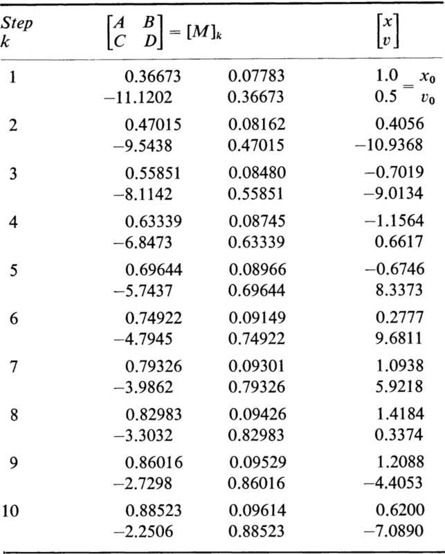
The values of hk, wk, and the elements of the matrices [M]k are tabulated in Table 3. The matrices [M]k and the values of xk and υk of the solution at the end of the kth subinterval as a result of the initial conditions x0 = 1 and ![]() are given in Table 4. The matrix [M] is obtained by the multiplication of the chain of matrices in the form
are given in Table 4. The matrix [M] is obtained by the multiplication of the chain of matrices in the form
As a consequence of (30.11), we have

The stability criterion (29.20) indicates that the solution is unstable. A table of hyperbolic functions gives the following value for a:
The solution at the end of n periods of the function F(t) is given by (29.15) with the value given by (30.13) for a.
If Hill’s equation has the form
throughout the fundamental interval ![]() it may be solved in this interval by means of Bessel functions1 in the form
it may be solved in this interval by means of Bessel functions1 in the form
where Jn and Yn are Bessel functions of the first and second kinds of order n1 and the A’s are arbitrary constants. If we let
and compute the derivative
it is evident that we may write x(t) and ![]() (t)= v in the convenient matrix form
(t)= v in the convenient matrix form
The Wronskian, Eq. (28.5), now takes the form
From the theory of Bessel functions1 we have the following result:
If this is substituted into (31.6), we obtain
The matrix [M] of (28.15) now becomes
The conditions for stability are given by (29.20) and the solution after n periods is given by
If k = 4π and ![]() Eq. (31.1) reduces to the one discussed in Sec. 30 by another method.
Eq. (31.1) reduces to the one discussed in Sec. 30 by another method.
As a final example of the general method, consider the solution of Hill’s equation (27.1) when the function F(t) has the form of a sawtooth wave as shown in Fig. 32.1. The function F(t) has the form
in the fundamental interval and repeats the variation at intervals of T. Hill’s equation now takes the form
in the fundamental interval. Let
This change of variable transforms (32.2) into the form
Equation (32.4) is a form of Stokes’s equation. The linearly independent solutions of this equation have been tabulated.1 The solution of (32.4) may also be expressed in terms of Bessel functions of order one-third2 in the following form:
where the A’s are arbitrary constants and
Fig. 32.1
In the notation of Sec. 28 we have
By the use of the recurrence relation of the theory of Bessel functions1
the following derivatives may be calculated:
Hence the solution of (32.2) in the fundamental interval ![]() expressed in the following form:
expressed in the following form:
Let the following notation be introduced:
The Wronskian W0 of (28.5) in this case is given by
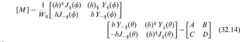
The matrix [M] of (28.15) is now
Hence
The stability conditions for the solution are given by (29.20) and the magnitude of the solution after n periods is given by (28.19) in terms of the initial conditions.
If b is large so that
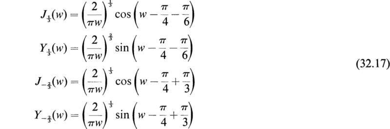
then terms of the order of ![]() can be neglected and the various Bessel functions involved may be represented by the dominant term of their asymptotic expansions. If this is done, we have
can be neglected and the various Bessel functions involved may be represented by the dominant term of their asymptotic expansions. If this is done, we have
If the Bessel functions in (32.13) and (32.14) are represented by their dominant terms (32.17), the following expressions are obtained for W0 and [M]:
and
In this case we have
and the stability criterion (29.20) may be easily applied.
The natural manner by which equations of the Mathieu-Hill type may be solved in terms of given initial conditions by the use of matrix algebra has been demonstrated. The powerful matrix notation and the use of Sylvester’s theorem to raise the matrices involved to the required powers greatly facilitate the solution of equations of this type.
The general theory of electrical circuits whose component parameters are linear and constant has been extensively developed and is well understood. In recent years, considerable attention and effort has been directed to the analysis and performance of circuits whose parameters vary with the time. Many of the most important and interesting problems of circuit theory involve variable parameters. For example, the equivalent circuits of the microphone transmitter, the condenser microphone, the induction generator, the super-regenerator, and many other practical devices contain parameters that are time-varying. Many systems in mechanical and acoustical engineering in which the compliance or the inertia parameters vary with the time lead to the same mathematical formulation of their behavior as do the time-varying circuit problems.
The analyses of electrical and mechanical systems involving time-varying parameters have been undertaken by many investigators using mathematical techniques. It is the purpose of this discussion to present four distinct mathematical methods that have been found useful for the analysis of such systems in the hope that an expository account of these techniques will prove useful to workers in this field of investigation.
The differential equations that determine the current or charge distribution of several time-variable circuits of practical importance are first-order linear equations of the following form:
where P(t) and F(t) are given functions of the time t. The initial conditions of these circuits are usually of such form that the dependent variable y(t) has the following initial value:
The general solution of (35.1), subject to the initial condition (35.2), is
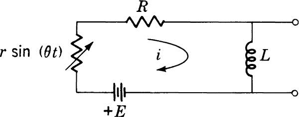
This general solution of (35.1) is very useful in the solution of many time-variable circuits of practical importance. As an example of the use of (35.3), consider the circuit of the carbon microphone shown in Fig. 35.1.1 The equivalent circuit of this device consists of a constant potential source E in series with a constant resistance R, a constant inductance L, and a time-varying resistance r sin(θt). The output terminals of the carbon microphone appear across the inductance of the circuit.
The differential equation satisfied by the current of the circuit of Fig. 35.1 is
This differential equation has the same form as (35.1) with y = i and F(t)= E/L. In this case, the integral ∫ P(t)dt is given by
where b = R/L, a = r/θL.
If the initial conditions of the circuit are i(0) = 0, the current is given by (35.3) in the following form:
The harmonic components of the current may be obtained by the well-known result in the theory of Bessel functions :2
where In(a) is the modified Bessel function of the first kind of order n. These functions have been extensively tabulated.3
Fig. 35.1
The modified Bessel functions have the following property:
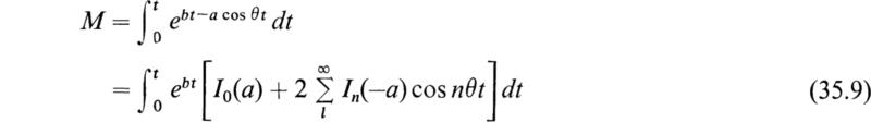
In order to obtain the various modulation products of the current from the general solution (35.6), it is necessary to evaluate the following integral:
This integral may be evaluated by the use of the following well-known result:
where
By the use of this result, the following expression for M may be obtained:
If these results are substituted into (35.6), the circuit current i(t) may be expressed in the following form:
This expression gives the steady-state and transient current of the microphone circuit. The modulation products of the steady-state solution may be readily computed by the use of this result.
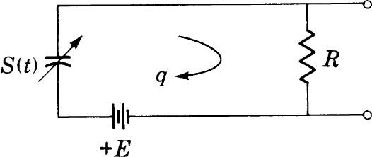
Another circuit of practical importance whose analysis leads to a differential equation of the form (35.1) is the equivalent circuit of the condenser transmitter.1 The equivalent circuit of this device is shown in Fig. 35.2. This circuit consists of a variable elastance parameter of the form S(t)= S0(1+k sin θt), where k < 1 in series with a constant potential source E and a constant resistance R. The output voltage of this device is taken from the
Fig. 35.2
terminals of the resistance R. The differential equation satisfied by the mesh charge q of this circuit is
This equation is of the form (35.1). If the initial condition of the circuit is q(0) = 0, the mesh charge is given by (35.3) in the form
where m = S0/R, n = kS0/θR.
The modulation products may be obtained by using (35.7) and performing the indicated integration. The response of other time-varying circuits whose equations are of first order may be obtained in a similar manner.
The response and stability of linear time-varying circuits that contain parameters whose magnitudes vary in a periodic manner with the time may be obtained by a matrix multiplication technique.1 This method of analysis is applicable when the differential equation governing the charge or current distribution of the circuit can be written as a Mathieu-Hill differential equation having the form
in which F(t) is a given periodic function of the time t and suitable initial conditions are prescribed.
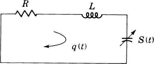
To illustrate this general mathematical technique, consider the circuit illustrated by Fig. 36.1. This circuit consists of a constant resistance and inductance parameters R and L in series with a time-varying capacitance whose elastance parameter is S(t). It is desired to determine the behavior of the circulating charge q(t) when the periodic variation of S(t) and the initial circuit charge q0 and current i0 of the circuit are prescribed at t = 0.
Fig. 36.1
Since there is a possibility of energy being furnished to the circuit by the agent that is causing the time variation of the capacitor, this circuit is said to be parametrically excited.1
The differential equation that determines the mesh charge q(t) of this circuit is
It will be assumed that the elastance S(t) is a periodic function of the time of fundamental period T so that
The initial conditions of the circuit will be assumed to be given by the equations
To simplify (36.2) it is convenient to introduce the new variable x(t) by the following substitution:
In terms of x(t), (36.2) is transformed into
where the function F(t) is given by
The initial conditions (36.4) may be expressed as initial conditions on x(t) by the following equations:
Since S(t) is a periodic function of fundamental period T, the function F(t) is also a periodic function having the same period. The interval from t = 0 to t = T is therefore the fundamental interval of the variation of F(t). Let u1(t) and u2(t) be two linearly independent solutions of (36.6) in the fundamental interval ![]()
The values of x(t)= x1, and its first derivative ![]() (t) = x2 may be expressed in the following form:
(t) = x2 may be expressed in the following form:
where K1 and K2 are arbitrary constants. It is convenient to write (36.9) as the single matrix equation
To simplify the writing, the following notation will be introduced:
In terms of this notation, (36.10) may be expressed in the following concise form:
The Wronskian1 W0 of the two solutions u1(t) and u2(t) is a constant in the fundamental interval ![]() and is the following determinant:
and is the following determinant:
Since the two solutions u1(t) and u2(t) are linearly independent, W0≠ 0. The matrix [u(t)] is therefore nonsingular and has the following inverse:
at t = 0, (36.12) becomes
hence
This equation determines the arbitrary constants in terms of the initial conditions. If this value of [K] is now substituted into (36.12) the result is
At the end of the fundamental interval t = T, the solution is given in terms of the initial conditions by the following equation:
or
where
It is easy to see that as a consequence of the periodicity of F(t) expressed by the equation
(36.6) is invariant to the change of variable
It is thus apparent that a solution of the form (36.17) may be obtained in each interval ![]() The final values of x1 and x2 at the end of one interval of the variation of F(t) are the initial values of x1 and x2 in the following interval. Therefore the solution at the instant t = 2T is
The final values of x1 and x2 at the end of one interval of the variation of F(t) are the initial values of x1 and x2 in the following interval. Therefore the solution at the instant t = 2T is
At the end of n fundamental periods of F(t), t = nT, the solution is
The solution at the time t = nT+ τ is
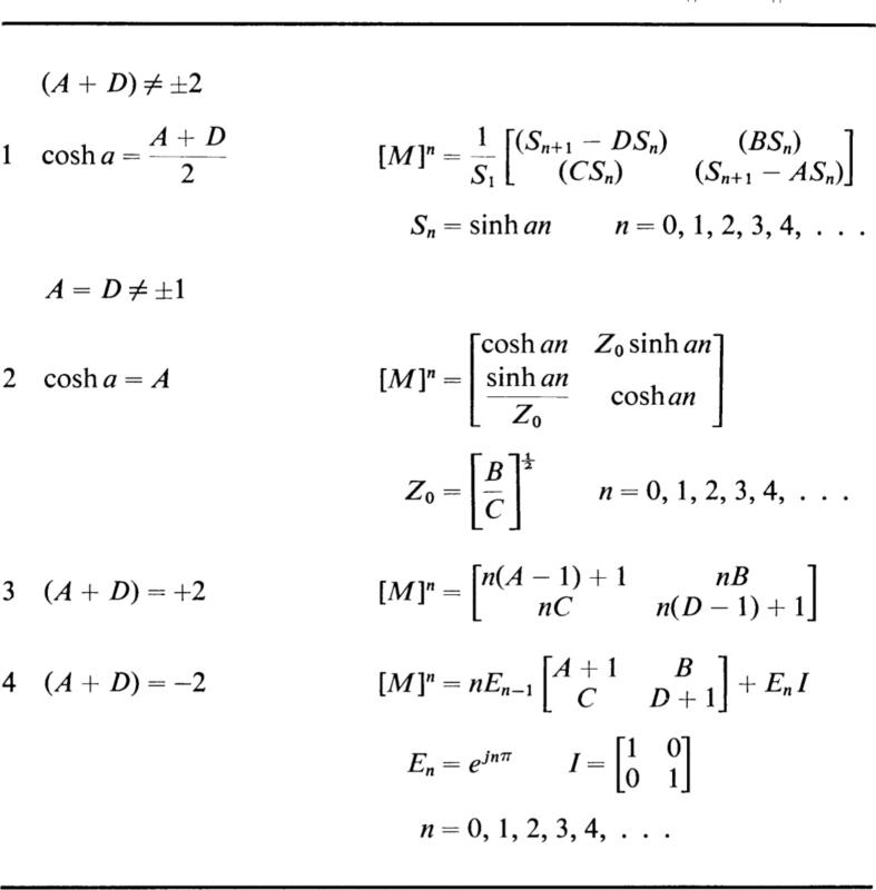
The solution of (36.6) is given by (36.25). The practical use of this solution depends on having an efficient technique for the computation of positive integral powers of the matrix [M]. These required powers of [M] are easily obtained by the use of Sylvester’s theorem of matrix algebra.1 Results are summarized in Table 5.
To illustrate the general method of solution, consider the case in which the elastance parameter S(t) of the circuit of Fig. 36.1 varies in the manner illustrated by Fig. 36.2. In this case the function F(t) has the following values:
It is easy to show that in this case (36.18) takes the following form:
where
![]()
The matrix [M] of (36.20) now takes the form
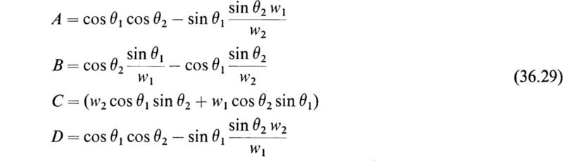
If the indicated matrix multiplication in (36.28) is performed, the following values are obtained for the elements A, B, C, D of the matrix [M]:
Fig. 36.2
Table 5 Positive integral powers of 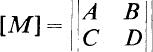
The values of x and ![]() after the end of n complete periods the square wave S(t) are given by
after the end of n complete periods the square wave S(t) are given by
The magnitudes of the circulating charge and the current of the circuit at t = nT may be obtained by the use of (36.5) and are given by
The powers of [M]n of the matrix [M] may be easily computed by the use of Table 5.
The nature of the charge and current oscillations of the circuit depend on the form taken by the high powers of the matrix [M]. In the usual case, A + D ≠ 2 and the matrix [M]n is given by the first entry of Table 5. In this case, the circuit charge at t = nT is given by (36.31) in the form
where Sn = sinh (an), and x1(0) and x2(0) are given in terms of the initial conditions of the circuit by (36.8). An examination of (36.32) shows that for large values of n, the charge q(nT) will grow indefinitely with n if
and the solution will be unstable. If, on the other hand,
q(nT) will eventually be damped out by the resistance and the circuit will be stable. If a = bT, steady oscillations of the circuits can be maintained by the energy source that is varying the elastance.
Since
it can be seen that the oscillations of the charge and the current of the circuit will grow indefinitely with time and the circuit therefore will be unstable if the circuit parameters are such that
The special cases in which A + D = ±2 lead to the forms for [M]n given in the third and fourth entries of Table 5 and may be treated similarly.
The matrix method is applicable when a solution of (36.6) in the interval ![]() is readily obtained and is particularly useful if the circuit has a parameter that undergoes square-wave or sawtooth variations. Additional examples of this method of solution are available.1, 2
is readily obtained and is particularly useful if the circuit has a parameter that undergoes square-wave or sawtooth variations. Additional examples of this method of solution are available.1, 2
A great many time-variable circuits that occur in practice have the property that the variable parameters involved exhibit only small variations about alarge average value. The fundamental differential equations of such circuits can usually be transformed so that they take the following general form:
where F(t) involves the driving potential of the circuit. If no external driving potentials are applied to the circuit, F(t)= 0, and (37.1) reduces to the homogeneous equation
If G2(t) is a real positive function that exhibits small variations about a large average value, it can be shown that1, 2
where A and B are arbitrary constants and ϕ(t) is given by
is a very good approximate solution of (37.2). More precisely, it can be shown1, 2 that if the variations of G(t) are such that
in the range in t under consideration, y(t) is an excellent approximation to the solution of (37.2). This approximation is known in the literature of mathematical physics as the Brillouin-Wentzel-Kramers (BWK)approximation. It has been used extensively in problems of quantum mechanics.3
As a first example of the use of the BWK approximation in the analysis of time-varying circuits, consider the circuit of Fig. 37.1. This is a series circuit that consists of a constant inductance L in series with a time-varying capacitance C(t) whose magnitude is
Fig. 37.1
The differential equation that is satisfied by the circulating charge q(t) of the circuit is
This is the differential equation of the equivalent circuit of a condenser microphone in which a sound wave of angular frequency 2θ is caused to vary the distance d between the two plates of a capacitor so that d= d0(1 — 2h cos 2θt) where d0 is the average distance of separation of the plates of the capacitor. Typical values of the various parameters in the case of radio-frequency modulation are
It is therefore justifiable to neglect terms of the order h2 and higher powers of h. Equation (37.7) is a special case of (37.1) with
provided that terms of h2 and higher are neglected. Since in this case G(t) performs small amplitude oscillations about the large average value w0, the inequality (37.5) is satisfied. The function ϕ(t) of (37.4) now takes the following form:
Therefore the BWK solution of (37.7) is
where A and B are arbitrary constants and c = w0h/2θ.
In order to determine the various harmonic components of the charge oscillations of the circuit, these expansions involving Bessel functions may be used:1
where the Jn(x) functions are Bessel functions of the first kind and nth order. If the quantity h in the square-root term of (37.11) is neglected, and Eqs. (37.12) are used, then, after certain algebraic reductions, (37.11) may be written in the form
where K0 and b are arbitrary constants. This solution of Eq. (37.7) was obtained by J. R. Carson by an entirely different procedure.1
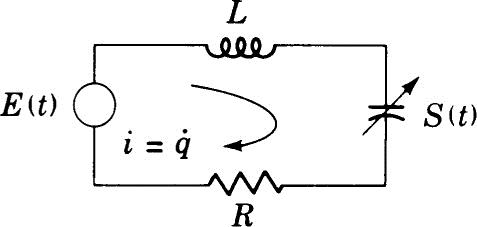
As a second example of the use of the BWK procedure, consider the circuit of Fig. 37.2. This circuit consists of a series connection of a resistance R, a constant inductance L, and a time-varying elastance S(t) in series with a periodic electromotive force E(t)= Emsin(wt). Let it be assumed that the variation of the elastance is of the form
where ![]()
S0 is the large average value of the elastance, and h is a small amplitude parameter. The differential equation satisfied by the circulating charge of the circuit of Fig. 37.2 is
To simplify the form of (37.15), introduce the notation
and the two variables x(t) and y(t) defined by the following equations:
In terms of the new variables x and y, (37.15) takes the form
Fig. 37.2
If the resistance of the circuit R is small, then ![]() and the term b2 may be neglected in (37.18). The complementary function of the differential equation (37.18) is the solution of the equation
and the term b2 may be neglected in (37.18). The complementary function of the differential equation (37.18) is the solution of the equation
This equation has the same form as (37.2). If the quantity h is so small that it can be neglected in comparison with unity, the BWK solution of (37.19) can be written in the form
where A1 and A2 are arbitrary constants and the functions y1(x) and y2(x) are given by
The general solution of (37.18) for the forced oscillations of the circuit may now be obtained by the method of variation of parameters1 in the form:
where F(x) is the right member of (37.18) given by
and W is the Wronskian of the solutions of (37.19) whose value is
for the case in which ![]() The terms containing the arbitrary constants in (37.22) constitute the complementary function of (37.19) and the terms involving the integrals give the particular integral of the equation.
The terms containing the arbitrary constants in (37.22) constitute the complementary function of (37.19) and the terms involving the integrals give the particular integral of the equation.
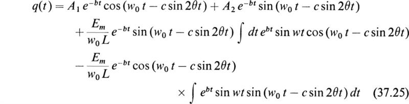
The approximate general solution of (37.15) may now be obtained by expressing (37.22) in terms of the original variables q and t. It has the form
The arbitrary constants A1 and A2 of the transient part of the solution may be evaluated if the initial conditions of the circuit at t = 0 are given. The harmonic content of the steady-state solution may be obtained by expanding the integrands as a series of harmonic terms by means of Eqs. (37.12) and integrating term by term. Further examples of the BWK method applied to the solution of the differential equations of time-varying circuits have been found.1
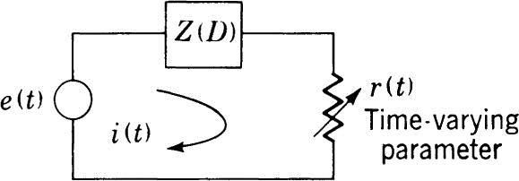
The Laplace-transform technique which has proved so useful in the analysis of linear circuits with constant parameters may be used to obtain useful results in the analysis of time-variable circuit problems. In order to illustrate the use of the Laplace-transform method in the analysis of time-varying circuits, consider the circuit of Fig. 38.1. This circuit is a series combination of a constant component whose operational impedance is Z(D), D = d/dt, in series with a time-varying resistance r(t) and a potential source e(t).
The differential equation that expresses the potential balance of this circuit may be written in the following operational form:
In order to formulate this equation as an integral equation let the following Laplace transforms be introduced:
Fig. 38.1
Let it be assumed that initially the circuit is at rest so that at t = 0, i(0) = 0, and q(0) = 0. That is, the initial current i(t) and the charge q(t) of the circuit are both zero at t = 0. With these initial conditions, the Laplace transform of (38.1) is given by
or
For simplicity, introduce the notation
With this notation (38.6) may be written in the following form:
Let the inverse Laplace transform of H(s) be h(t), so that
The current of the circuit i(t) is therefore obtained by taking the inverse transform of I(s) in the form
If the Faltung or convolution theorem of the Laplace-transform theory is applied to the right-hand member of (38.10), the following result is obtained:
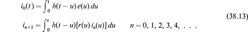
This is an integral equation of the Volterra type. Volterra1 has shown that the solution of (38.11) is given by the following series of functions:
where
The series (38.12) may be shown to be a rapidly convergent one. The i0(t) term represents the current in the circuit without the presence of the variable resistance element; the i1(t) term represents the first correction term caused by the resistance variation, etc.
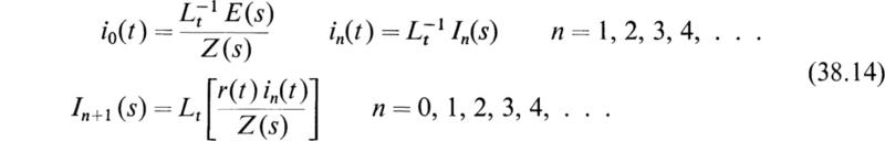
In the computation of the various functions in(t) of the series (38.12), it is frequently simpler to use the following equations:
As a special example consider a circuit whose constant part consists of a constant inductance L in series with a constant resistance R. In this case, Z(s) has the form
Let the applied potential be Emsin(wt) and the variable resistance have the form r(t) = r0 sin(θt) with r < R. Therefore,
The integral equation (38.11) now takes the form
The solution of this integral equation is
where
The transient and steady-state oscillations of the circuit may therefore be computed to the degree of accuracy desired.
If the time-varying circuit contains a variable inductance L(t) in series with a constant part of operational impedance Z(D), the circuit equation takes the following form:
If the circuit is at rest at t = 0, this equation can be transformed into the following Volterra-type integral equation:
where ![]()
The solution of (38.24) has the form (38.20) with
The case involving a variable capacitance may be treated in a similar manner. Further applications of the Laplace transform and the integral equation technique in the analysis of time-varying systems are available.1–4
The present state of the mathematical analysis of circuits with time-varying parameters may be compared with the status of alternating-current networks before the practical development and use of complex impedances and symbolic methods of solution. Although methods for obtaining the transient and steady-state solutions of these networks were available, yet the use of alternating-current networks by engineers and physicists proceeded in a halting manner until the mathematical methods for the analysis of problems involving these networks had been interpreted and systematized so that they could be readily applied to circuits in common practical usage.
The purpose of this discussion has been to catalogue some of the analytical methods that have been found useful in the analysis of time-varying systems and to interpret and systematize them for practical use. Unless existing methods and methods yet to be developed for the solution of problems involving these circuits are interpreted and systematized for practical use, the attempt to utilize time-varying circuits in practical work will be limited and severely circumscribed.
The general behavior of electrical circuits whose parameters are constants has been extensively studied and is well understood. In recent years, a great deal of attention has been paid to the general theory and performance of circuits whose parameters are functions of the time, especially when they vary periodically [30–38]. Examples of linear time-varying circuits of practical importance occur in the theory of electrical communications. Frequency modulation, for instance, utilizes variations of capacitance or, to a lesser degree, inductance. The microphone transmitter contains a variable resistance whose value is varied by some source of energy outside the circuit, and the capacitor microphone contains a variable capacitance. The introduction of superregeneration has especially stimulated an interest in circuits that contain periodic variation of a resistance parameter [39].
The mathematical analysis of the performance of electrical circuits whose parameters are periodic functions of the time leads generally to the solution of Mathieu’s and Hill’s differential equations. These equations have the following general form
where G2(x) is a periodic function of x and H(x) is a continuous function of x. Despite the vast amount of literature on the theory of Mathieu functions [40], it is still a formidable task to obtain rigorous solutions of Eq. (40.1) in cases of practical importance, and approximate methods must be employed.
The great majority of linear time-varying circuits that occur in communications engineering have the property of the variable parameters involved exhibiting only small variations about a large average value. In such cases a very good approximate solution of Eq. (40.1) can be obtained by a method used by Brillouin, Wentzel, and Kramers to solve equations of the type
in connection with problems of wave mechanics [41, 42]. Although the BWK method was used by Brillouin, Wentzel, and Kramers to solve problems in wave mechanics in 1926, the procedure is a very old one and the first indication of its use is found in the collected papers of the eminent mathematician Liouville, published in 1837.
To determine the type of approximation involved in the BWK procedure, consider the following function:
where ![]() is the base of the natural logarithms, C1 and C2 are arbitrary constants, and j = √–l. The function ϕ>(x) is given by
is the base of the natural logarithms, C1 and C2 are arbitrary constants, and j = √–l. The function ϕ>(x) is given by
By direct differentiation of Eq. (41.2), it can be shown that this function satisfies the following differential equation:
If G2(x) is a periodic function that exhibits only small variations about a large average value, it can be shown that
throughout the range in x, and hence that Eq. (41.2) is an approximate solution of Eq. (41.1).
In the case where G2(x) is a positive periodic function of x, Eq. (41.2) may be written in the alternative form
where A and B are arbitrary constants, and ϕ(x) is given by (41.3). Equation (41.6) is the usual BWK approximate solution of Eq. (41.1).
As a first example of the use of the general BWK procedure, consider the circuit of Fig. 42.1. This is a series circuit that consists of a constant inductance L in series with a capacitance C(t) that varies with time in such a manner that
where C0 and h are constant parameters with ![]() If q denotes the charge on the capacitance, the differential equation of the circuit is
If q denotes the charge on the capacitance, the differential equation of the circuit is
Typical values of the various parameters in the case of radio-frequency modulation are
It is therefore justifiable to neglect terms containing h2 and higher and write
Consequently Eq. (42.2) may be written in the following form:
If the new variables, y = q and x =pt, are introduced, Eq. (42.7) takes the following form:
This equation is a special case of Eq. (41.1) with
Fig. 42.1
provided that terms of order h2 and higher are neglected. Since ω0/p = 2 × 10⁴ and h = 2 × 10⁻⁴, it can be seen that Eq. (41.5) is satisfied and an accurate approximate solution of Eq. (42.8) is given by Eq. (41.6). In this case we have
Therefore the BWK solution of Eq. (42.8) is
where A and B are arbitrary constants and a = ω0/p and c = ω0h/2p.
To determine the various harmonic components, the following expansions involving Bessel functions [43] may be used:
where the Jn(a) functions are Bessel functions of the first kind and the nth order. With the aid of Eq. (42.12), (42.11) may be written in the following form after certain algebraic reductions:
where K and θ are arbitrary constants. This is the BWK solution of Eq. (42.7) for the circuit charge. If the quantity h in the square-root term of Eq. (42.13) is neglected in comparison with unity, this equation may be written in the form
where K0 and θ are arbitrary constants. Equation (42.14) is a less accurate solution of (42.6) and was obtained by Carson [44] by a different procedure.
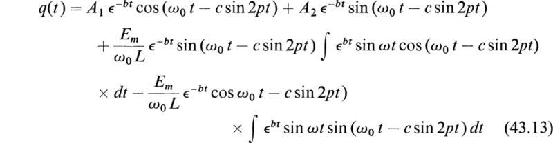
As a second example of the use of the BWK procedure, consider the circuit of Fig. 43.1. This circuit consists of a series connection of a constant resistance R, a constant inductance L, and a time-varying elastance S(t) in series with a periodic electromotive force E(t)= Emsinωt. Let it be assumed that the variation of the elastance is of the form
Fig. 43.1
S0 is the constant part of the elastance, and h is a small amplitude parameter. The differential equation satisfied by the charge q on the elastance is
Let
and introduce the new variable y(t) by means of the transformation
In terms of these parameters, Eq. (43.2) may be written in the form
Let x=pt; then Eq. (43.5) becomes
If the resistance R of the circuit is small, then ![]() and the terms b2 may be neglected in Eq. (43.6). The complementary function of the differential equation (43.6) is the solution of the equation
and the terms b2 may be neglected in Eq. (43.6). The complementary function of the differential equation (43.6) is the solution of the equation
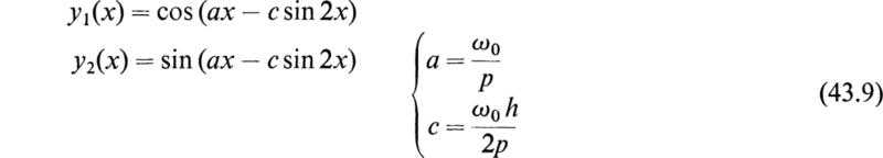
This is Eq. (42.9), and its BWK solution is given by Eq. (42.11). If h is small, it can be neglected in comparison with unity in the square-root term of Eq. (42.11), and the general solution of (43.7) may be written in the form
where A1 and A2 are arbitrary constants and functions y1(x) and y2(x) are given by
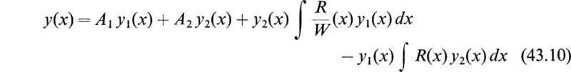
The general solution of Eq. (43.6) for the forced oscillations of the circuit of Fig. 43.1 may now be obtained by the method of the variation of parameters [16] in the following form:
where R(x) is the right member of Eq. (43.6) given by
and W is the Wronskian of the solutions, Eq. (43.12), whose value is
for the case in which ![]() The terms containing the arbitrary constants in Eq. (43.10) constitute the complementary function of (43.6), and the terms involving the indefinite integrals give the particular integral of the equation. The approximate general solution of Eq. (43.2) may now be obtained by expressing Eqs. (43.4) and (43.12) in terms of the original variables. It has the following form:
The terms containing the arbitrary constants in Eq. (43.10) constitute the complementary function of (43.6), and the terms involving the indefinite integrals give the particular integral of the equation. The approximate general solution of Eq. (43.2) may now be obtained by expressing Eqs. (43.4) and (43.12) in terms of the original variables. It has the following form:
The arbitrary constants A1 and A2 of the transient part of the solution may be evaluated if the initial conditions of the circuit at t = 0 are given. The harmonic content of the steady-state solution may be obtained by expanding the integrand as a series of harmonic terms by means of Eq. (42.12) and integrating term by term.
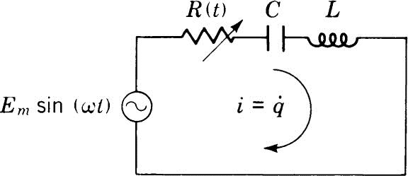
In recent years, the introduction of superregeneration has stimulated an interest in the study of circuits that involve a periodic variation of the resistance parameter [7]. Consider the circuit of Fig. 44.1. This circuit consists of a constant inductance and capacitance in series with a periodically varying resistance R(t). It is assumed that a harmonic forcing potential E(t)= Emsin(ωt) is impressed on the circuit.
Fig. 44.1
The circulating charge of this circuit satisfies the following differential equation
Let the resistance parameter have the following periodic variation:
Let
with
and introduce the transformation
This transformation transforms Eq. (44.1) into the following equation:
If Eq. (44.2) is substituted into Eq. (44.6) and terms of the order k2 are neglected, the result is
where
If b is small, ![]() and the cos(pt) term in Eq. (44.7) may be neglected. The complementary function of Eq. (44.7) is then the solution of
and the cos(pt) term in Eq. (44.7) may be neglected. The complementary function of Eq. (44.7) is then the solution of
Let x = pt. In the variable x, Eq. (44.9) is transformed into
The function G(x) (of the section on BWK approximation) is now given by
where
The function ϕ(x) is in this case given by
Two linearly independent BWK solutions of Eq. (44.10) are
By the method described in Sec. 43 and after some algebraic reductions, the following approximate general solution of Eq. (44.1) may be obtained:
The quantities A1 and A2 are the arbitrary constants of the transient part of the solution, and the terms involving the integrals give the steady-state response of the system to the BWK order of approximation.
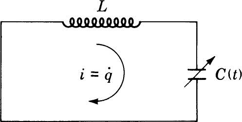
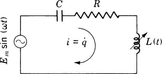
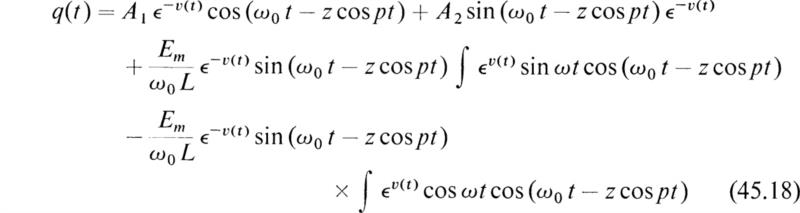
As a final example of the BWK method, consider the circuit of Fig. 45.1. This circuit consists of a constant resistance and capacitance in series with a periodically varying inductance parameter. The circuit is energized by a periodic electromotive force E(t) = Em sin ωt.
Fig. 45.1
The differential equation satisfied by the charge on the capacitance is [8]
where ϕ is the total magnetic flux linking the circuit, R is the resistance, and C the capacitance of the circuit. The flux ϕ is related to the inductance of the circuit by the fundamental equation
Hence if Eq. (45.2) is substituted into (45.1), the following equation is obtained:
If the indicated differentiation is carried out, then
This equation may be written in the following form:
where
Let
then Eq. (45.5) is transformed into
Let it now be assumed that the variable inductance has the following form:
If Eq. (45.10) is substituted into Eqs. (45.6), (45.7), and (45.9) and terms in a2 are neglected, then after some algebraic reductions Eq. (45.9) may be written in the following form:
where
By the transformation x=pt, Eq. (45.11) may be transformed into the form
By the BWK method discussed in Sec. 41, the following complementary function of Eq. (45.15) yc may be obtained:
where
A1 and A2 in Eq. (45.16) are arbitrary constants. The method of the variation of parameters, discussed in Sec. 43, gives the following approximate general solution of Eq. (45.4) with the inductance variation equation (45.10):
The transient part of the solution contains the arbitrary constants, and the integral terms contain the steady-state response. The harmonic content of the steady-state response may be obtained by using the Bessel function expansions (42.12) and term by term integration.
The analysis presented in this discussion is an attempt to apply the method of the BWK approximation, which has yielded very useful and interesting results in problems of wave mechanics to the analysis of linear circuits whose parameters vary periodically with the time. A survey of the literature of circuit analysis reveals that this powerful method of analysis has been neglected by the electrical engineers, and it is hoped that this presentation will given an impetus to its future use for the solution of problems involving linear time-varying parameters.
1. Given the second-order linear differential equation,
![]()
where F(x) is a slowly varying positive function of x. Show that the substitution x = ejϕ(x) leads to the following nonlinear differential equation of the Ricatti type:
![]()
Obtain an approximate solution of the Ricatti equation, and show that
![]()
where ϕ(x) = ∫ F(x)dx and A and B are arbitrary constants, is the approximate solution of the original equation (Brillouin-Wentzel-Kramers approximation).
2. A body of mass m falls through a medium that opposes its fall with a force proportional to the square of its velocity so that its equation of motion is
![]()
where x is the distance of fall and υ is the velocity. If, at t = 0, x = 0, and υ = 0, find the velocity of the body and the distance it has fallen at a time t. Plot the phase trajectory of the motion.
3. Solve Bernoulli’s equation
![]()
subject to the initial condition x = x0 at t = 0.
4. Given the differential equation

where w0, h, A, B, w1, and w2 are constants. Devise a method of successive approximations for the solution of this equation. Let the initial conditions be x = x0 and ![]() at t = 0. (This equation1 is the basis of Helmholtz’s theory of combinations of tones.)
at t = 0. (This equation1 is the basis of Helmholtz’s theory of combinations of tones.)
5. A particle oscillates in a straight line under the action of a central force tending to a fixed point O on the straight line and varying as the distance from O. If the motion takes place in a medium that resists the motion with a force proportional to the square of the velocity of the particle, find the relation between the amplitudes of any two successive arcs on each side of O. Plot the phase trajectory of the motion.
6. The nonlinear resistive material thyrite has a voltage-current characteristic of the form V = Bib, where V is the potential difference applied across the thyrite resistor, i the current, B a constant that depends on the length and cross section of the resistor. The parameter b has the value 0.28. An electrical circuit is composed of a linear inductor L and a thyrite resistor in series with a harmonic electromotive force. The equation of the circuit is
![]()
Obtain an approximate expression for the steady-state periodic current of this circuit.
7. Show that the solution of the differential equation
![]()
with the initial conditions dx/dt = 0, x = x0, at t = 0, is

This is the equation of motion of a particle undergoing a restoring force which increases exponentially with the displacement.
8. Show that ![]() is the exact solution of the differential equation
is the exact solution of the differential equation
![]()
This is a special case of a phenomenon called frequency demultiplication by van der Pol.1
9. Show that, if the motor of the motor-generator oscillator of Fig. 16.1 is replaced by a large capacitor and the rest of the system is left unchanged, the current will execute relaxation oscillations.
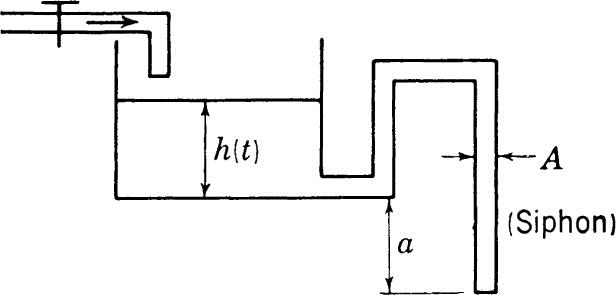
10. Discuss the oscillations of the height h(t) of the level of water in the tank of Fig. P. 10. Does h(t) execute relaxation oscillations ? Plot the phase trajectory of h(t).
Fig. P 10
11. Given the differential equation
![]()
Determine a solution of this equation of the form
![]()
where A(t) and B(t) are slowly varying functions of t. Assume that ![]() wB, and d2A/dt2 = d2B|dt2 = 0.
wB, and d2A/dt2 = d2B|dt2 = 0.
12. Solve the linear equation
![]()
for small values of μ, by the method of Kryloff and Bogoliuboff.
13. Show that the differential equation
![]()
has the approximate solution x = x0 sinwt, where the angular frequency w is given by ![]() . J1(x0) is the Bessel function of the first kind and first order. If
. J1(x0) is the Bessel function of the first kind and first order. If ![]() the above equation governs the motion of a simple pendulum of length L.
the above equation governs the motion of a simple pendulum of length L.
14. The forced oscillations of a simple pendulum are governed by the equation

Show that the first approximation for the periodic motion is given by θ = Asin wt, where the amplitude A satisfies the equation A(1 – w2/k2) – F/k2 = A – 2J1 (A), where J1(A) is the Bessel function of the first kind and first order.
15. A particle of mass m moves along the x axis under the action of a restraining force F(x) = 1/x2 – 1/x. Show that, if the motion of the mass is started with a small amount of energy E0, the motion will be oscillatory. If, however, the motion is started with a large amount of energy E, show that the motion is not periodic and extends to infinity. Determine the critical energy that forms the dividing line between the two cases. Draw the phase trajectories for the oscillatory and nonoscillatory cases.
16. A pendulum (Froude’s pendulum) is suspended from a dry horizontal shaft, of circular cross section, by a ring. It is well known that, if the shaft rotates with a suitable constant angular velocity w0, the pendulum oscillates with a gradually increasing amplitude which reaches a final ultimate value. Write the differential equation of motion of this pendulum, and use it to explain the above phenomenon.
(HINT: Assume the frictional force at the suspension to be a function of w0 – θ, the difference between the angular velocity of the shaft and the pendulum.)
17. Devise a graphical method for the solution of the equation
![]()
subject to the initial conditions x = a and ![]() at t = 0.1
at t = 0.1
18. The differential equation of an oscillator whose motion is retarded by viscous and Coulomb friction and is being driven by a harmonic force is
![]()

The term ![]() represents the effect of dry friction. Obtain an approximate expression for the periodic-steady-state solution of this equation.1
represents the effect of dry friction. Obtain an approximate expression for the periodic-steady-state solution of this equation.1
1. McLachlan, N. W.: “Ordinary Nonlinear Differential Equations in Engineering and Physical Science,” 2d ed., Oxford University Press, New York, 1956. (This book contains an excellent discussion of the better-known analytical procedures and an extensive bibliography of 211 titles covering the international literature to 1950.)
2. Stoker, J. J.: “Nonlinear Vibrations,” Interscience Publishers, Inc., New York, 1950. (Contains a clear exposition of the topological methods for solving autonomous systems and a fairly complete discussion of stability.)
3. Andronow, A. A., and C. E. Chaikin: “Theory of Oscillations,” Princeton University Press, Princeton, N.J., 1949. (Contains a clear and interesting exposition of the topological properties of many autonomous systems.)
4. Minorsky, N.: “Introduction to Nonlinear Mechanics,” J. W. Edwards, Publisher, Inc., Ann Arbor, Mich., 1947. (An extensive survey of the international literature to 1947; a clear discussion of topological methods, analytical methods, nonlinear resonance, and relaxation oscillations.)
5. von Kármán, T.: The Engineer Grapples with Nonlinear Problems, Bulletin of the American Mathematical Society, vol. 46, no. 8, pp. 615–683, 1940. (An excellent exposition of self-excited nonlinear oscillations, subharmonic resonance, large-deflection theory, elasticity with finite deformations, fluid jets, waves and finite amplitudes, viscous fluids, and compressible fluids; contains excellent bibliographies on these fields.)
6. Kryloff, N., and N. Bogoliuboff: “Introduction to Nonlinear Mechanics,” Princeton University Press, Princeton, N.J., 1943. (A clear and careful exposition of the Kryloff-Bogoliuboff method, with interesting applications to electrical circuits and dynamics.)
7. Duffing, G.: “Erzwungene Schwingungen bei veranderlicher Eigenfrequenz und ihre technische Bedeutung,” Vieweg-Verlag, Brunswick, Germany, 1918. (A pioneer study of nonlinear vibration problems; discusses methods of approximation and questions of stability with technical applications.)
8. Lefshetz, S.: “Contributions to the Theory of Nonlinear Oscillations,” vol. II, Princeton University Press, Princeton, N.J., 1952. (Discussions of several topics of nonlinear differential equations by several mathematicians from the rigorous point of view.)
9. Pipes, L. A.: “Operational Methods in Nonlinear Mechanics,” Department of Engineering, University of California, Los Angeles, 1951. (Contains some useful methods for the solution of certain classes of nonlinear technical problems; operational methods are introduced to reduce the algebraic labor of the solution.)
10. Edson, W. A.: “Vacuum-tube Oscillators,” John Wiley & Sons, Inc., New York, 1953, pp. 408–412.
11. McLachlan, N. W.: “Theory and Application of Mathieu Functions,” Oxford University Press, London, 1947. (Contains 226 references to the international literature.)
12. Kemble, E. C: “The Fundamental Principles of Quantum Mechanics,” McGraw-Hill Book Company, New York, 1937, pp. 90–112. (Contains a detailed exposition of the BWK procedure and an extensive list of references to papers on wave mechanics.)
13. McLachlan, N. W.: “Bessel Functions for Engineers,” Oxford University Press, London, 1934, pp. 42–43.
14. Ford, L. R.: “Differential Equations,” McGraw-Hill Book Company, New York, 1933, pp. 75–76.
The bibliographies in the above books and reports are quite extensive and cover the most important papers to 1950. The following technical papers are representative of recent publications in the field of nonlinear problems:
15. Sim, A. C.: A Generalization of Reversion Formulae with Their Application to Non-linear Differential Equations, Philosophical Magazine, ser. 7, vol. 42, pp. 237–240, March, 1951. (Discusses an ingenious method for the approximate solution of nonlinear differential equations similar to the reversion of a power series.)
16. Cartwright, M. L.: Forced Oscillations in Nonlinear Systems, Journal of Research of the National Bureau of Standards, vol. 45, no. 6, December, 1950. (A rigorous discussion of the van der Pol equation with a forcing term.)
17. Hayashi, C.: Forced Oscillations with Nonlinear Restoring Force, Journal of Applied Physics, vol. 24, no. 2, pp. 198–207, 1953. (An excellent discussion of forced oscillations of nonlinear systems; the equation is transformed so that topological methods can be used.)
18. Hayashi, C.: Stability Investigation of the Nonlinear Periodic Oscillations, Journal of Applied Physics, vol. 24, no. 3, pp. 238–246, 1953. (The stability of nonlinear periodic oscillations is discussed by solving the variational equation for small deviations from the periodic state.)
19. Hayashi, C.: Subharmonic Oscillations in Nonlinear Systems, Journal of Applied Physics, vol. 24, no. 5, pp. 521–529, 1953. (The possibility of subharmonic solutions and their stability is studied for systems having a nonlinear restoring force and driven by a harmonic forcing function.)
20. Pipes, L. A.: A Mathematical Analysis of a Series Circuit Containing a Nonlinear Capacitor, Communication and Electronics, July, 1953, pp. 238–244. (An extension of Duffing’s method and its application to a technically important problem.)
21. Pipes, L. A.: Applications of Integral Equations to the Solution of Nonlinear Electric Circuit Problems, Communication and Electronics, September, 1953, pp. 445–450. (The formulation of some nonlinear differential equations in terms of integral equations and their solution by iterative procedures.)
22. Thomsen, J. S.: Graphical Analysis of Nonlinear Circuits Using Impedance Concepts, Journal of Applied Physics, vol. 24, no. 11, pp. 1379–1382, 1953. (An interesting extension of linear-impedance concepts to the calculation of the amplitudes of nonlinear oscillations.)
23. Jacobsen, L. S.: On a General Method of Solving Second Order Ordinary Differential Equations by Phase-plane Displacements, Journal of Applied Mechanics, vol. 19, no. 4, pp. 533–553, December, 1952. (This paper presents a powerful graphical procedure for the solution of complicated equations; the method is illustrated by several important examples.)
24. Klotter, K.: Nonlinear Vibration Problems Treated by the Averaging Method of W. Ritz, Proceedings of the First National Congress of Applied Mechanics, pp. 125–131, American Society of Mechanical Engineers, 1952.
25. Clauser, F. H.: The Behavior of Nonlinear Systems, Journal of the Aeronautical Sciences, vol. 23, no. 5, pp. 411–434, May, 1956. (An excellent expository paper. It presents a diversified group of nonlinear phenomena in terms of fundamental and well-understood concepts. Contains a comprehensive bibliography of recent papers.)
26. van der Pol, B.: Nonlinear Theory of Electric Oscillations, Proceedings of the Institute of Radio Engineers, vol. 22, pp. 1051–1086, 1934.
27. Cartwright, M. L.: Forced Oscillations in Nearly Sinusoidal Systems, Proceedings of the Institution of Electrical Engineers, vol. 95, pt. Ill, pp. 88–96, 1948.
28. Gillies, A. W.: The Application of Power Series to the Solution of Nonlinear Circuit Problems, Proceedings of the Institution of Electrical Engineers, vol. 96, pt. Ill, pp. 453–475, 1949.
29. Tucker, D. G.: Forced Oscillations in Oscillator Circuits and the Synchronization of Oscillators, Journal of the Institution of Electrical Engineers, vol. 92, pt. Ill, p. 226, 1946.
30. Pipes, L. A.: The Reversion Method of Solving Nonlinear Differential Equations, Journal of Applied Physics, vol. 23, p. 202, 1952.
31. Pipes, L. A.: A Mathematical Analysis of a Dielectric Amplifier, Journal of Applied Physics, vol. 23, no. 8, pp. 818–824, August, 1952.
32. Miles, James G.: Bibliography of Magnetic Amplifier Devices and the Saturable Reactor Art, Transactions of the American Institute of Electrical Engineers, vol. 70, pt. II, pp. 2104–2123, 1951.
33. Finzi, L. A., and Pitman, G. F., Jr.: Comparison of Methods of Analysis of Magnetic Amplifiers, Proceedings of the National Electronics Conference, vol. 8, p. 144, 1952.
34. Pipes, L. A.: Operational and Matrix Methods in Linear Variable Networks, Philosophical Magazine, vol. 25, pp. 585–600, 1938.
35. Barrow, W. L.: On the Oscillations of a Circuit Having a Periodically Varying Capacitance, Proceedings of the Institute of Radio Engineers, vol. 22, pp. 201–212, 1934.
36. Erdelyi, A.: Ueber die Freien Schwingungen in Kondensatorkreisen mit Periodisch Veralnderlicher Kapazitaet, Physica, vol. 5, no. 19, pp. 585–622, 1934.
37. Pipes, L. A.: Solution of Variable Circuits by Matrices, Journal of the Franklin Institute, vol. 224, pp. 767–777, 1937.
38. Bennett, W. R.: A General Review of Linear Varying Parameter and Nonlinear Circuit Analysis, Proceedings of the Institute of Radio Engineers, vol. 38, pp. 259–263, 1950.
39. Kingston, R. H.: Resonant Circuits with Time-Varying Parameters, Proceedings of the Institute of Radio Engineers, vol. 37, pp. 1478–1481, 1949.
40. Bura, P., and Tombs, D. M.: Resonant Circuit with Periodically-Varying Parameters, Wireless Engineer, pp. 95–100, April 1952, pp. 120–126, May, 1952.
41. Gadsen, C. P.: An Electrical Network with Varying Parameters, Quarterly of Applied Mathematics, vol. 8, no. 2, pp. 199–205, 1950.
42. Aseltine, J. A.: Transforms for Linear Time-Varying Systems, Report No. 52.1, University of California, Los Angeles, February, 1952.
43. Brillouin, L.: The B.W.K. Approximation and Hill’s Equation, Quarterly of Applied Mathematics, vol. 7, no. 4, pp. 363–380, 1950.
44. Carson, J. R.: Notes on the Theory of Frequency Modulation, Proceedings of the Institute of Radio Engineers, vol. 10, no. 62, 1922.
1 B. van der Pol and M. J. O. Strutt, Philosophical Magazine, vol. 5, p. 18, 1928.
1 Fraser et al., op. cit.
1 E. Kamke, “Differentialgleichungen Lösungsmethoden und Lösungen,” p. 442, Chelsea Publishing Company, New York, 1948.
1 N. W. McLachlan, “Bessel Functions for Engineers,” Oxford University Press, London, 1941.
1 “Tables of the Modified Hankel Functions of Order One-Third and of Their Derivatives,” Harvard University Press, Cambridge, Mass., 1945.
2 Kamke, op. cit.
1 N. W. McLachlan, “Bessel Functions for Engineers,” Oxford University Press, London, 1941.
† Reprinted from the Transactions of the IRE Professional Group on Circuit Theory, vol. CT-2, no. 1, March, 1955.
1 E. A. Guillemin, “Communication Networks,” vol. I, pp. 403–416, John Wiley & Sons, Inc., New York, 1931.
2 W. G. Bickley, “Bessel Functions and Formulae,” pp. 15–17, Cambridge University Press, London, 1953.
3 E. Jahnke and F. Emde, “Tables of Functions,” pp. 137–138, Dover Publications, Inc., New York, 1943.
1 E. A. Guillemin, op. cit.
1 L. A. Pipes, Matrix Analysis of Linear Time-varying Circuits, Journal of Applied Physics, vol. 25, pp. 1179–1185, September, 1954.
1 N. Minorsky, “Introduction to Nonlinear Mechanics,” pp. 362–369, J. W. Edwards, Publisher, Incorporated, Ann Arbor, Mich., 1947.
1 L. R. Ford, “Differential Equations,” pp. 115–117, McGraw-Hill Book Company, New York, 1933.
1 R. A. Frazer, W. J. Duncan, and A. R. Collar, pp. 79–80, “Elementary Matrices,” Cambridge University Press, London, 1938.
1 L. A. Pipes, Matrix Solution of Equations of the Mathieu-Hill Type, Journal of Applied Physics, vol. 24, pp. 902–910, July, 1953.
2 L. Brillouin, “Wave Propagation in Periodic Structures,” pp. 125–127, Dover Publications, Inc., New York, 1953.
1 L. Brillouin, A Practical Method for Solving Hill’s Equation, Quarterly of Applied Mathematics, vol. 6, pp. 167–178, July, 1948.
2 L. Brillouin, The B.W.K. Approximation and Hill’s Equation, Quarterly of Applied Mathematics, vol. 7, pp. 363–380, January, 1950.
3 E. C. Kemble, “The Fundamental Principles of Quantum Mechanics,” pp. 90–112, McGraw-Hill Book Company, New York, 1937.
1 W. G. Bickley, “Bessel Functions and Formulae,” pp. 15–17, Cambridge University Press, London, 1953.
1 J. R. Carson, Notes on the Theory of Frequency Modulation, Proceedings of the Institute of Radio Engineers, vol. 10, pp. 57–64, February, 1922.
1 L. R. Ford, op. cit.
1 L. A. Pipes, Analysis of Linear Time-varying Circuits by the Brillouin-Wentzel-Kramers Method, Transactions of the AIEE, Communication and Electronics, no. 11, pp. 93–96, March, 1954.
1 V. Volterra, “Leçons sur les Équations Intégrales,” Gauthier-Villars, Paris, France, 1913.
1 J. R. Carson, Theory and Calculation of Variable Electric Systems, Physics Review, vol. 17, pp. 116–134, February, 1921.
2 J. R. Carson, “Electric Circuit Theory and the Operational Calculus,” pp. 159–173, McGraw-Hill Book Company, New York, 1926.
3 V. Bush, “Operational Circuit Analysis,” pp. 338–358, John Wiley & Sons, Inc., New York, 1927.
4 L. A. Pipes, Operational and Matrix Methods in Linear Variable Networks, Philosophical Magazine, ser. 7, vol. 25, pp. 585–600, April, 1938.
† A reprint from Communication and Electronics, published by American Institute of Electrical Engineers. Copyright 1954 and reprinted by permission of the copyright owner. The Institute assumes no responsibility for statements and opinions made by contributors.
1 See L. A. Pipes, An Operational Treatment of Nonlinear Dynamical Systems, Journal of the Acoustical Society of America, vol. 10, pp. 29–31, July, 1938.
1 B. van der Pol, Frequency Demultiplication, Nature, vol. 120, p. 363, 1927.
1 See Lord Kelvin, On Graphic Solutions of Dynamical Problems, Philosophical Magazine, vol. 34, pp. 332–348, 1892.
1 See J. P. Den Hartog, Forced Vibrations with Combined Coulomb and Viscous Friction, Transactions of the American Society of Mechanical Engineers, vol. 53, pp. 107–115, 1931.