In many branches of engineering and physics, processes are encountered which are not known with exactness. In the study of phenomena of this type, the applications of the methods of statistics and of the theory of probability are imperative. In this chapter, some of the basic elementary concepts and methods employed in the theory of statistics and probability will be given. The notion of probability is a very difficult concept whose fundamental aspects we shall not discuss. Simple cases and examples will be given to introduce its use in a reasonable way. For the reader who wishes to study the vast subject of statistics and probability further, a fairly complete and representative set of references to the more important modern treatises on the subject is given at the end of the chapter.
When a series of measurements is made on a set of objects, the set of objects being measured is called a population. A population may be, for example, the animals living on a farm, the group of people living in a certain city, the automobiles produced by a factory in a year, the set of results of a physical or chemical experiment, etc.
If a single quantity is measured for each member of a population, this quantity is called a variate. Variates are usually denoted in the mathematical literature by symbols such as x or y. The possible observed values of a variate x will be a finite sequence or set of numbers x1 x2, x3, . . . , xn. The numbers xk, for example, may be the heights of a group of n individuals or the prices of a certain make of automobile in a dealer’s showroom.
In a given population, the number of times a particular value xr of a variate is observed is called the frequency fr of xr. For example, an automobile dealer may have nine cars in his showroom; three cars are priced at $3,500, four at $4,000, and two at $2,000. In this case we have x1 = $3,500, f1 = 3, x2 = $4,000, f2 = 4, and x3 = $2,000, f3 = 2. The total number of automobiles in the population is N, where
The total value of the automobiles S is
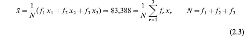
The average or mean price ![]() is
is
The most elementary statistical quantity defined by a distribution is the arithmetic mean ![]() of the variate x, usually known as the mean. This is the sum of the values of x for each member of the population divided by N. Therefore,
of the variate x, usually known as the mean. This is the sum of the values of x for each member of the population divided by N. Therefore,
Let us suppose that a is a typical value of the variate x, and let us define
It is thus evident that dr is the deviation of xr from the typical value a. The variate d has a distribution fr over the values dr. The mean ![]() of d for this distribution is
of d for this distribution is
![]() is simply related to
is simply related to ![]() ; this can be seen by writing (2.6) in the form:
; this can be seen by writing (2.6) in the form:
Therefore we have
The following relation is sometimes useful.
Equation (2.8) is useful in computing ![]() quickly, provided that we choose a to be a number close to the mean.
quickly, provided that we choose a to be a number close to the mean.
In statistical investigations, it is of interest to know whether or not a distribution is closely grouped around its mean. One of the most useful quantities for estimating the spread of a distribution is the standard deviation σ. Before we define σ it is instructive to note that ![]() as given by (2.7) is the first moment of a distribution about a given value a of the variate. We note from (2.8) that if
as given by (2.7) is the first moment of a distribution about a given value a of the variate. We note from (2.8) that if ![]() , then the first moment
, then the first moment ![]() .
.
The second moment ![]() of a distribution about a given value a of the variate is the average over the population of the squares of the differences dr = xr – a between a and the values of the variate xr. It is given by
of a distribution about a given value a of the variate is the average over the population of the squares of the differences dr = xr – a between a and the values of the variate xr. It is given by
It is apparent that if most of the measured values of x for the population are approximately equal to ![]() will be small, while if a differs considerably from the observed values of x, then
will be small, while if a differs considerably from the observed values of x, then ![]() will be large since all the terms in (3.1) are positive. If we now take
will be large since all the terms in (3.1) are positive. If we now take ![]() in (3.1), that is, we take the second moment about the mean
in (3.1), that is, we take the second moment about the mean ![]() of the population, this second moment μ2 is called the variance. The variance is therefore given by
of the population, this second moment μ2 is called the variance. The variance is therefore given by
The variance gives an estimate of the spread of values of x about their mean. The variance is not directly comparable to ![]() since it is of dimension of x2.
since it is of dimension of x2.
The positive square root of μ2 is the standard deviation σ; since it is of the same dimension as x σ gives us an estimate of the spread of values of x which can be compared directly with ![]() . By definition, we have therefore
. By definition, we have therefore
where we have made use of (2.9).
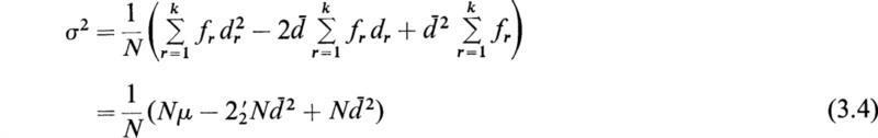
If (3.3) is expanded, we obtain the following result:
It is thus evident that the variance μ2 and the second moment ![]() about any value a are related by
about any value a are related by
In order to calculate the standard deviation σ, it is usually easier to calculate the second moment ![]() about a simple value a and then use (3.5) instead of using (3.3) directly.
about a simple value a and then use (3.5) instead of using (3.3) directly.
Since σ2 is the mean value of the squares of the deviations of the variate from its average value ![]() , σ (the “root mean square”) gives us an over-all measure of the deviation of the set from the average
, σ (the “root mean square”) gives us an over-all measure of the deviation of the set from the average ![]() without reference to sign. There are two other features of the population which are sometimes found useful. Suppose that a frequency diagram has been constructed in which the ordinates represent the number of readings lying in successive intervals. The interval in which the ordinate attains its maximum clearly corresponds to the most frequent or “most fashionable” value of x among the set. This value is called the mode; in general, it is not identical with the average or mean, but it will be if the frequency curve is symmetric about the mean value. A frequency curve may have more than one mode, but we are here concerned only with cases in which a single mode exists.
without reference to sign. There are two other features of the population which are sometimes found useful. Suppose that a frequency diagram has been constructed in which the ordinates represent the number of readings lying in successive intervals. The interval in which the ordinate attains its maximum clearly corresponds to the most frequent or “most fashionable” value of x among the set. This value is called the mode; in general, it is not identical with the average or mean, but it will be if the frequency curve is symmetric about the mean value. A frequency curve may have more than one mode, but we are here concerned only with cases in which a single mode exists.
We may also arrange our data in ascending order to magnitude and divide them into two sections halfway, so that as many measurements lie about this division as below it. This position is called the median, and is such that it is useful in analyzing the data in many experimental observations.
Let us take an ordinary coin and flip it N times. Let the number of times the “heads” side of the coin comes up be denoted by Nh; we may then write the following ratio:
When this experiment is performed with a balanced coin, the result of this experiment has been found to be that
Because of the result (4.2), we say that the probability of a coin coming up heads when it is flipped is ![]() .
.
This simple case can be generalized to the following situation. Consider an experiment that is performed N times. Let the times that the experiment succeeds be Ns; then if the ratio
approaches the limit
we say that the probability of the success of the experiment is Ps.
Because in this case the probability Ps is measured by performing the experiment and is not predicted, Ps is called the a posteriori probability that the experiment will be successful.
Let us now perform another experiment that has n equally likely outcomes. Let us call the successes of the experiment ns. If we now predict that the ratio
Then ps is called the a priori probability that the experiment will succeed.
Of course, the two types of probability should always give the same answer. If the a posteriori probability comes out to be different from the a priori probability, it will be concluded that an error has been made in the analysis. In the following discussion, no distinction will be made between the two types of probability.
In this section a simple discussion of the fundamental laws of probability will be given. Let P(A) be the probability of an event called A occurring when a certain experiment is performed. By the definition of probability, P(A) is a fraction that lies between 0 and 1. We also have by definition that if
the event A is certain to happen. However if,
the event A is certain not to happen.
To illustrate more complex possibilities, let us consider an experiment with N equally likely outcomes that involve two events A and B. Let us use the following notation:
n1 = the number of outcomes in which A only occurs
n2 = the number of outcomes in which B only occurs
n3 = the number of outcomes in which both A and B occur
n4 = the number of outcomes in which neither A nor B occurs.
N = n1 +n2 + n3 + n4
We see that by the use of the above notation we may define the following probabilities:
From the above definitions, we see that
or
We also have
or
If A and B are mutually exclusive events so that the occurrence of one precludes the occurrence of the other, then the probability of their joint occurrence is zero and we have
For this case (5.10) reduces to the equation
If the events A and B are statistically independent, then the probability of the occurrence of A does not depend on the occurrence of B and vice versa; we then have
In this case, Eq. (5.12) reduces to
If the events A and B are statistically independent, then the additive law of probability (5.10) becomes
As an example of the use of (5.17), let it be required to compute the probability that when one card is drawn from each of two decks, at least one will be an ace. In this case the events A and B are the drawing of an ace out of a deck of 52 cards. Therefore,
Since the events A and B are statistically independent, we have from (5.17) the following result:
Some interesting relations among conditional probabilities may be deduced by means of Eq. (5.12). If we solve (5.12) for P(B/A), we obtain
However, we also have from (5.12) the result
If we substitute this into (5.20), we obtain
Let us now write a relation similar to (5.22) but with B replaced by C. We thus obtain
We now divide Eq. (5.22) by (5.23) and obtain the result
This result is a form of Bayes’s theorem in the theory of probability.
In Sees. 2 and 3 we discussed observed or empirical distributions. The theory of probability is concerned with the prediction of distribution when some basic law is assumed to govern the behavior of the variate. A simple example of a law of probability is that governing the behavior of a perfect die. The fact that the die is symmetric with respect to its six faces suggests very strongly that each of the faces is equally likely to end facing upward if we make an unbiased throw of the die. The probability p of any particular face appearing is thus equal to ![]() . A similar situation is that involving the probability p that a particular card is on top of a thoroughly shuffled pack of 52 cards,
. A similar situation is that involving the probability p that a particular card is on top of a thoroughly shuffled pack of 52 cards, ![]() . The fact that if a fair die is thrown, the probability distribution is
. The fact that if a fair die is thrown, the probability distribution is ![]() for k = 1, 2, . . . , 6 is the definition of a fair die. The statistical problem then becomes one of deciding whether or not any particular die is fair.
for k = 1, 2, . . . , 6 is the definition of a fair die. The statistical problem then becomes one of deciding whether or not any particular die is fair.
When a card is drawn, a die is thrown, or the height of a man selected from a certain group of men is measured, we are said to be making a trial. Let us make a series of completely independent trials on a system, and let there be a finite number n of possible results of a trial. Let these n possible results be denoted by x1 x2, x3, . . . , xn. If in the series of trials the result x1 occurs m1 times, the result x2 occurs m2 times, and in general the result xr occurs mr times (r, 2, 3, ... , n), then
Now if as N becomes large, it is found that the proportion of any result xr measured by xr/N tends to a definite value pr, so that
then pr is the probability of the result xr.
Since we cannot in practice make an infinite number of trials, we cannot determine pr exactly by making a series of trials. It is therefore evident that a law of probability that specifies definite values of the probabilities pr is never established with certainty by a series of trials, although it may be strongly suggested. The assumption of a law of probability corresponding to a series of trials is therefore a hypothesis which may or may not be confirmed by further trials.
If we divide (6.1) by N, we obtain
We now let N → ∞ in (6.3) and use the result (6.2) to obtain
As an example of the above discussion, we note that the possible results of a throw of a die are x1 = 1, x2 = 2, x3 = 3, x4 = 4, x5 = 5, x6 = 6. For an unbiased die, we assume the probability law ![]() . If in a large number of throws the values of mr/N (r = 1, 2, 3, . . . , 6) do not tend to the value
. If in a large number of throws the values of mr/N (r = 1, 2, 3, . . . , 6) do not tend to the value ![]() , we conclude that the die is biased.
, we conclude that the die is biased.
As an example of the use of an assumed law of probability let us consider the following question: “What is the probability that the face number 1 appears at least once in n throws of a die?”
Since we assume that the probability of the face 1 appearing in one throw is ![]() , the probability of not obtaining a 1 in one throw is
, the probability of not obtaining a 1 in one throw is ![]() The probability of not obtaining a 1 in two throws is
The probability of not obtaining a 1 in two throws is ![]() and of not obtaining a 1 in n throws is
and of not obtaining a 1 in n throws is ![]() . The probability of throwing a 1 at least once in n throws p is therefore
. The probability of throwing a 1 at least once in n throws p is therefore ![]() In this calculation we assume that the result of each throw is independent of the result of any other throw and use (5.16).
In this calculation we assume that the result of each throw is independent of the result of any other throw and use (5.16).
Since the mathematical theory of probability treats questions involving the relative frequency with which certain groups of objects may be conceived as arranged within a population, it is necessary to review the theory involving the number of ways in which various subgroups may be partitioned from the members of a larger group.
In dealing with objects in groups one is led to consider two kinds of arrangements, according to whether the order of the objects in the groups is or is not taken into account. Some elementary results in the theory of combinations and permutations will now be reviewed.
The number of arrangements, or permutations, of n objects is n!. This can be seen as follows since the first position can be occupied by any of the n objects, the second by any of the n – 1 remaining objects, etc. Therefore if we denote the number of permutations of n objects by nPn we have
where n! = (1)(2)(3) · · · (n – 1)n is the factorial of n. By definition, 0! = 1 and 1! = 1.
The number of permutations of n different things taken r at a time is denoted by the symbol nPr and is found easily as follows. The first place of any arrangement may have any one of the n things, so that there are n choices for the first place. The second place may have any one of the remaining n – 1 things, the third any of the remaining (n –2), and so on, to the rth place which has any of the remaining (n –r + 1). It follows that
The combinations of n things taking r at a time is defined as the possible arrangements of r of the n things, no account being taken of the order of the arrangement. Thus the combinations of three things a, b, c, taking two at a time, are ab, ac, and bc. The combination ba is the same as ab, and so on.
The number of combinations of n things taking r at a time is denoted by the symbol nCr and is found as follows. Any combination of the r things can be arranged in r! ways since this is the number of arrangements of r things taking r at a time, or rPr. If every combination is so treated, we clearly obtain nPr arrangements and it therefore follows that
If we divide (7.3) by r!, we obtain
The quantity nCr = n!/r!(n – r)! is called the binomial coefficient, it is shown in works on algebra that if n is a positive integer, we may write
Equation (6.5) for n = 2, 3, 4, . . . , is known as the binomial theorem.
The following interesting and useful properties of the binomial coefficient nCr can be established:
As a simple example of the use of Eq. (7.4), let it be required to solve the following problem. There are n points in a plane, no three being on a line. Find the number of lines passing through pairs of points.
We may solve this problem by realizing that since no three points lie on a line, any line can be considered as a combination of two of the n points. The number of lines is therefore nC2 = n!/2! (n – 2)!=n(n – l)/2.
In many phases of the mathematical theory of probability, the factorial of large numbers occurs. A classical result given by Stirling is of paramount importance in the computation of the factorial of large numbers. The formula given by Stirling was obtained in the 1730s and may be stated in the following form:
The percent error of this formula for finite values of n is of the order of 100/12n percent error.
In addition to being a very useful method for the computation of factorial numbers, Stirling’s formula is very useful in a theoretical sense. Its use in the computation of the factorial or large numbers may be seen by considering the computation of 10!. Instead of multiplying together a large number of integers, we have merely to calculate the factorial by the use of expression (8.1) by means of a table of logarithms, this involves far fewer operations. For example, for n = 10 we obtain the value 3,598,696 by Stirling’s expression (using seven-figure tables), while the exact value of 10! obtained by direct multiplication is 3,628,800. The percentage error obtained by the use of Stirling’s formula is of the order of ![]() percent too low.
percent too low.
A more exact formula for the computation of factorial numbers is the following one:
It is thus evident that the expressions n! and ![]() differ only by a small percentage of error when the value of n is large. The factor
differ only by a small percentage of error when the value of n is large. The factor ![]() gives us an estimate of the degree of accuracy of the approximation.
gives us an estimate of the degree of accuracy of the approximation.
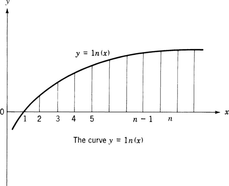
In order to obtain this remarkable formula let us try to estimate the area under the curve y = ln x. This curve has the general form depicted in Fig. 8.1. If we integrate ln x by parts we obtain the result
An is the exact area under the curve shown in Fig. 8.1.
If we erect ordinates y1 y2, . . . , yn at x = x1 x = x2, . . . , x = xn, the trapezoidal rule for the area under the curve Tn gives
Fig. 8.1
Since we have
we obtain the following expression for Tn on substituting (8.5) into (8.4):
By the definition of the factorial number n!, we have
Therefore if we take the natural logarithm of (8.7), we obtain
If we now compare (8.6) with (8.8) it can be seen that
The exact area An and the approximate area Tn are of the same order of magnitude. Since the trapezoids used in computing Tn lie below the curve y = 1n (x), it is apparent that the true area An exceeds the trapezoidal area Tn. Let us write
If we solve (8.10) for ln(n!), we obtain
Let us write
We therefore have as a consequence of (8.11) and the definition of the natural logarithm the result
It can be shown that the quantity an is bounded and is a monotonic increasing function of n. Therefore the quantity bn is bounded and is a monotonic decreasing function of n. It can be shown that†
If we substitute (8.12) into (8.13), we obtain the result
This is Stirling’s result. For finite values of n, (8.15) gives a result for n! that is of the order of 100/12n percent too small. For more precise results, the inequality (8.2) may be used. The factor ![]() gives us an estimate of the degree of accuracy of the approximation.
gives us an estimate of the degree of accuracy of the approximation.
In many problems encountered in the mathematical theory of probability, the possible values of a variate x are not discrete but lie in a continuous range. For example, the heights of adults normally take values in the continuous range from 4.5 to 6.5 ft. Even though observed heights are classified as taking one of a finite discrete set of values, any theoretical probability law should refer to the continuous range. If, for example, a law of probability predicted a distribution of heights at intervals of ![]() in., it would not be appropriate and adequate for comparison with a set of measurements made to the nearest centimeter.
in., it would not be appropriate and adequate for comparison with a set of measurements made to the nearest centimeter.
A law of probability for a continuous variate is therefore expressed in terms of a probability function ϕ(x), such that ϕ(x)dx is the probability of a trial giving a result in the infinitesimal range [x – (dx/2), x + (dx/2)] for all values of x. The probability P(x1,x2) of the result lying between values x1 and x2 is then
Since the total probability is unity, we have
where the integral is taken over the complete range of the variate x. The equation (9.1) is analogous to Eq. (7.4) for discrete distributions; integration over the probability function replaces summation over the discrete probabilities.
The results of Sees. 2 and 3 apply equally well to probabilities. The mean of a probability distribution for a variate x is called the expectation E(x) and is defined by
Since the sum of the probabilities is unity, we have
Therefore the expectation E(x) as given by (10.1) takes the form
The expectation of a probability distribution of a continuous variate is defined by the equation
where the integration takes place over the whole range of x.
The second moment about a of a discrete probability distribution ![]() is defined by the equation
is defined by the equation
The second moment about a of a continuous probability distribution is defined by the equation
The variance μ2 is given by (10.5) or (10.6) with a = [x]. The standard deviation σ is given by
The standard deviation and the second moment ![]() are related in the same manner in (3.5) by the equation
are related in the same manner in (3.5) by the equation
where
so that
It is interesting to note that when a = [x], then (10.10) becomes
As an example of the above definitions consider the following illustration. Let us suppose that cards numbered 1, 2, 3, . . . , n are put in a box and thoroughly shuffled; then one card is drawn at random. If we assume that each card is equally likely to be drawn, so that the law of probability of drawing the cards is
then the expectation E(x) of the number x on the card is
The second moment about x = 0 of the probability distribution of x is, by (10.5),
The variance is given by (10.7) in the form
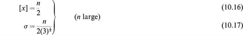
It can be seen that for large values of n we have
It is to be expected that the values of [x] and σ will become proportional to n when n is large.
As an example of a continuous distribution, consider a variatex which is equally likely to take any value in the range (0, X). In such a case the probability function ϕ(x) must equal a constant ϕ0 in this range and zero elsewhere. In order to satisfy (9.2), we must have
The expectation E(x) of x is, by (10.4),
The variance is given by (10.6) with a = [x] = X/2, so that
Therefore the standard deviation is ![]()
Let us consider a variate x with probability function f(x). Let μ be the mean value and σ the standard deviation of x. We shall prove that if we select any number a, the probability that x differs from its mean value μ by more than a is less than σ2/a2. This means that x is unlikely to differ from μ by more than a few standard deviations, and that therefore the standard deviation σ gives an estimate of the spread of the distribution. For example, if a = 2σ, we find that the probability for x to differ from μ by more than 2σ is less than ![]()
Proof By the definition of the standard deviation σ, we have
If we now sum over values of x for which x exceeds (μ + a) = x0, we get less than σ2, so that we have
If we replace (x – μ) by a in (10.22), the sum is further decreased and we have
We may write (10.23) in the form
However f(x) is the sum of the probabilities of values of x which differ from μ by more than a, so that x > (μ + a) and (10.24) says that this probability is less than σ2/a2. This result is known in the literature as Chebyshev’s inequality.
Let us suppose that a trial can have only two possible results, one called a “success” with probability p, and the other called a “failure” with a probability of q = (1 – p). If we make n independent trials of this type in succession, then the probability of a particular sequence of r successes and (n – r) failures is p2qn–r. However, the number of sequences with r successes and (n – r) failures is
Therefore the probability of there being exactly r successes in n trials is
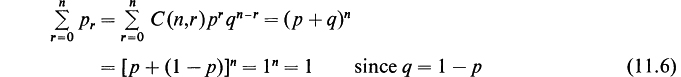
It will be noticed that P(r) is the term containing pr in the binomial expansion of (p+q)n. For this reason the probability distribution (11.2) is known as the binomial distribution.
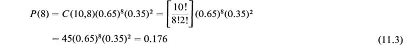
Example 1 If the probability that a man aged 60 will live to 70 is p = 0.65, what is the probability that 8 out of 10 men now aged 60 will live to 70? This is exactly the problem proposed above, with p = 0.65, r = 8, and n = 10. The answer is, therefore,
Example 2 What is the probability of throwing an ace exactly three times in four trials with a single die? In this case we have n = 4, r = 3, and since there is one chance in six of throwing an ace on a single trial, we have ![]() . Therefore we have
. Therefore we have
Example 3 What is the probability of throwing a deuce exactly three times in three trials? In this case ![]() , therefore we have the result
, therefore we have the result
![]()
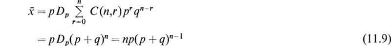
The expectation or the mean number of successes ![]() is given by equation (10.1) in the form
is given by equation (10.1) in the form
If we denote the partial derivative with respect to p by Dp, we note that
Since the denominator of (11.5) is unity, we have
The series in (11.8) is summed by treating p and q as independent variables. If we now use the result (11.7), we may write (11.8) in the form
We now substitute q = 1 – p in (11.9) and obtain the result
Therefore the mean number of successes for the binomial distribution is ![]()
We may compute the variance of the binomial distribution by the use of Eq. (10.8). The second moment ![]() about x = 0 of the distribution of the number of successes can be found by a method similar to that used in computing the first moment above (we leave the derivation as an exercise for the reader and quote the result):
about x = 0 of the distribution of the number of successes can be found by a method similar to that used in computing the first moment above (we leave the derivation as an exercise for the reader and quote the result):
As a consequence of (10.8) we have
Therefore the standard deviation of the total number of successes in n trials is
The Poisson distribution is derived as the limit of the binomial distribution when the number of trials n is very large and the probability of success p is very small. For the binomial distribution we have seen that the mean number of successes is given by
We now investigate the limiting form taken by the binomial distribution as the number of trials n tends to infinity and the probability p tends to zero in such a manner that
If we substitute p = m/n in the expression (11.2) for the binomial distribution, we obtain the equation
This expression may be written in the form
Now for any fixed r we have, as n tends to infinity,
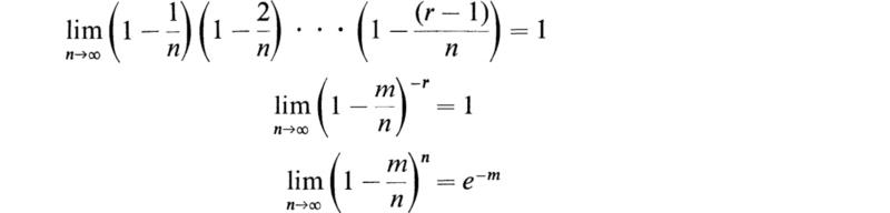
We therefore see that the limiting form of (12.4) as n tends to infinity is
This is known as the Poisson distribution.
We note that
as it should.
The mean ![]() of the Poisson distribution may be computed by the equation
of the Poisson distribution may be computed by the equation
The standard deviation of the Poisson distribution may be obtained by taking the limiting value of the standard deviation of the binomial distribution as we let p tend to zero. Equation (11.12) may be written in the form
We therefore have
Therefore,
We thus see that the standard deviation of the Poisson distribution is ![]()
A most important probability distribution that arises as a limit of the binomial distribution is a continuous distribution known as the normal or gaussian distribution, with the probability function
We shall show that μ is the mean of the distribution and σ is the standard deviation of the normal or gaussian distribution. If the function ϕ(x) is to be a probability density function, it is implied that
In order to verify that (13.2) is true, let us compute
In order to simplify (13.3), we make the substitution.
in the integral (13.3) and find that it is transformed into
From a table of definite integrals we obtain the result
If we now substitute (13.6) into (13.5), we find that A =1
We may compute the mean ![]() he normal distribution by the use of Eq. (10.4), which in this case takes the form
he normal distribution by the use of Eq. (10.4), which in this case takes the form
To simplify (13.7), let us introduce the following change in variable:
With this change in variable, (13.7) becomes
From a table of definite integrals, we have the results
If we substitute the results (13.10) into (13.9), we obtain
We have therefore verified that μ is the mean or expected value of the distribution ϕ(x)f (13.1).
The variance μ2 = σ2 of the normal distribution may be obtained by the use of (10.6) by placing a = μ and thus obtaining
If we now substitute ϕ(x) as given by (13.1) into (13.12) and make use of the change in variable
we obtain
The integral
may be integrated by parts to obtain
Fig. 13.1
If the above value for I is substituted into (13.14),
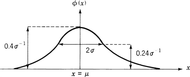
Therefore σ correctly represents the standard deviation of the normal or gaussian distribution (Fig. 13.1).
The maximum value of ϕ(x) is located at x = μ; ϕ(μ) is approximately ![]() When x = μ ± σ, the value of ϕ(x) is slightly less than
When x = μ ± σ, the value of ϕ(x) is slightly less than ![]() . It is easy to show that the points x = μ ± σ are the points of inflection of the normal distribution curve ϕ(x). It is of great interest to know the probability that the deviation y = x — μ from the mean is within certain limits. The probability that y lies between the limits σt1 and σt2 is
. It is easy to show that the points x = μ ± σ are the points of inflection of the normal distribution curve ϕ(x). It is of great interest to know the probability that the deviation y = x — μ from the mean is within certain limits. The probability that y lies between the limits σt1 and σt2 is
By placing t1 = –a and t2 = a in (13.18) and using a table of definite integrals, it can be shown that the probability that the deviation y exceeds 2σ is less than ![]() and the probability that y exceeds 3σ is of the order of 0.003. In statistics, an observation which is improbable is said, to be significant. For a normally distributed variate, it is usual to regard a single observation with |x| > μ + 2σ as significant and one with |x| > μ + 3σ as highly significant.
and the probability that y exceeds 3σ is of the order of 0.003. In statistics, an observation which is improbable is said, to be significant. For a normally distributed variate, it is usual to regard a single observation with |x| > μ + 2σ as significant and one with |x| > μ + 3σ as highly significant.
The normal or gaussian distribution may be derived as a limiting form of the binomial distribution when n becomes very large and p remains constant.†
The normal or gaussian distribution (13.1) is sometimes also known as the normal error law, although some statisticians object that it is not in fact a normal occurrence in nature because it is only valid as a limiting case for exceptionally large numbers. Sufficiently large numbers are, however, available in problems of applied physics, such as the kinetic theory of gases and fluctuations in the magnitude of an electric current, and so the gaussian distribution seems more real to physicists and engineers than to social and biological scientists. It is interesting to note that the eminent mathematical
physicist H. Poincaré, in the preface to his “Thermodynamique”† makes the laconic remark, “Everybody firmly believes in the law of errors because mathematicians imagine that it is a fact of observation, and observers that it is a theorem of mathematics.”
The application of the gaussian distribution to the theory of errors is made reasonable by the fact that any process of random sampling tends to produce a gaussian distribution of sample values, even if the whole population from which the samples are drawn does not have a normal distribution. Hence it is usual to assume that the gaussian distribution will be a useful approximation to the distribution of errors of observation, provided that all causes of systematic error can be excluded.
The area under some part of the gaussian distribution function is frequently needed. That is, we must evaluate the integral of ϕ(x) between finite values of x. For example, let it be required to evaluate the integral I where
In order to simplify the above integral, let
With this change in variable, (13.19) becomes
where
Now the function F(z) given by
has been extensively tabulated. It is easy to see that the integral is given by
in terms of the function F(z).
As an interesting typical problem involving a statistical distribution, consider that the heights of 500 men are measured to the nearest ![]() in. The frequencies fr of heights xr (in inches) are given in the following table.
in. The frequencies fr of heights xr (in inches) are given in the following table.
Heights of 500 men
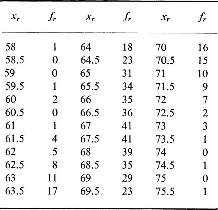
Show that the distribution of the heights of the 500 men given in the above table is approximately normal, with mean 67 in. and standard deviation 2.5 in. Assuming this normal distribution of heights, which of the following measurements of heights, considered individually, are significant or highly significant: 63 in., 72 in., 69.5 in., 58.5 in., 73 in., 75 in. ?
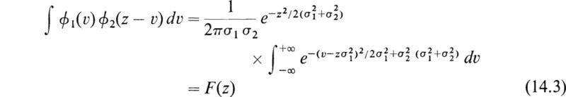
If two variates x and y are distributed normally, their sum u = x + y is also distributed normally. To prove this, we shall refer each distribution to its mean and assume that the distribution functions of ![]() are
are
The probability that (υ + w) takes a particular value z is found by integrating over the probabilities that υ and w take particular values summing to z. This gives
If we now let
the integral in (14.4) becomes
Hence the distribution (14.4) is
We therefore see that z = υ + w is normally distributed about the mean value zero, with standard deviation given by
The distribution of u = x + y, therefore, has the expectation ![]() with a standard deviation given by (14.8).
with a standard deviation given by (14.8).
Let x1 x2 …, xn be a set of n measurements. The xi i = 1, 2, . . . ,n, quantities may be the n determinations of the velocity of light in a certain medium. If we let z be a typical value of the measurements xi then di is the deviation of the measurement xi from z where
Let y represent the sum of the squares of the deviations of the measurements xi from the typical value z, so that
We now wish to choose the typical value z so that the sum of the squares of the deviations y is a minimum. We therefore minimize (15.2) in the usual way by computing the derivative
On setting the derivative dy/dz equal to zero and solving for z, we find
That is, we find that the arithmetic mean of the measurements xi is the typical value that minimizes y. It will be noted that ![]() gives the “best” typical value of the xi quantities in the least-square sense.
gives the “best” typical value of the xi quantities in the least-square sense.
The minimum value of y, ymin is obtained by substituting ![]() in (15.2) and thus obtaining
in (15.2) and thus obtaining
If we divide (15.5) by n, we obtain the variance σ2 of the set of measurements xi so that
The square root of (15.6) is the standard deviation a of the set of measurements xi so that
We now turn to a very important question that arises in the theory of statistics: “What is the relation between the standard deviation of the individual measurements and the standard deviation of the mean of a set of measurements?”
In order to answer this question, we will assume that we have a parent distribution of errors which follow the Gauss distribution. (The justification for assuming that the distribution is gaussian is that in practice errors do follow the gaussian law). We suppose first that we take N measurements or a sample of the parent distribution. We then take another sample or set of measurements. If we now compute the mean and standard deviation of both sets, these quantities will in general be different. That is, the mean and variance of a sample of N observations are not in general equal to the mean and variance of the parent distribution.
The process to be followed is to take M sets of N measurements, each with its own mean and standard deviation, and then compute the standard deviation of the means. The standard deviation of the means provides an indication of the reliability of any one of the means.
To facilitate the calculation let the following notation be introduced:
σ = the standard deviation of the individual measurements
σm = the standard deviation of the means (of the various samples)
xsi = measurement i in the set s
![]() = the mean of the set s
= the mean of the set s
![]() = the mean of all the measurements
= the mean of all the measurements
dsi = the deviation of xsi xsi – ![]() =dsi
=dsi
Dsi = ![]() = the deviation of the mean
= the deviation of the mean ![]()
Since we are taking M sets of measurements with N measurements in each set, there will be n = MN measurements in the total. The variance of the individual measurements is given by
The variance of the means is given by
The deviations Ds of the means can be expressed in terms of the deviations dsi of the individual observations as follows:
We also have
If we now substitute the square of (16.4) into (16.1), we obtain
The substitution of the square of (16.3) into (16.2) gives the results
After some reductions, it can be seen that (16.6) may be written in the following form:
If we now compare (16.5) with (16.7), we see that
or therefore
Therefore the variance of the mean of a set of N measurements is simply the variance of the individual measurements divided by the number of measurements.
It may be mentioned that in order to reduce (16.6) to the form (16.7) it is necessary to assume that the cross-product terms are negligibly small. This is true for the gaussian distribution, and since experimental measurements so often obey the gaussian distribution, formula (16.8) is a very useful one.
1. What is the probability that number 1 appears at least in n throws of dice ?
2. A hunter finds that on the average he kills once in three shots. He fires three times at a duck; on the assumption that his a priori probability of killing is ![]() what is the probability that he kills the duck?
what is the probability that he kills the duck?
3. Prove the following theorem: If in any continuously varying process a certain characteristic is present to the extent of one in T units, then the probability that the characteristic does not occur in a sample of t units is e–t/T. (Consider the Poisson distribution.)
4. It is known that 100 liters of water have been polluted with 106 bacteria. If 1 cc of water is drawn off, what is the probability that the sample is not polluted?
5. An aircraft company carries on the average P passengers M miles for every passenger killed. What is the probability of a passenger completing a journey of m miles in safety ?
6. Given the result of Prob. 5, estimate an apparently reasonable premium to pay in order that if a passenger is killed in such a flight, his heir would receive $10,000.
7. If during the weekend road traffic 100 cars per hr pass along a certain road, each taking 1 min to cover it, find the probability that at any given instant no car will be on this road. (NOTE : Evidently no car must have entered the road during the previous minute; however, on the average a car enters every 3,600/100 = 36 sec. It is thus apparent that the required probability is e–60/36.)
8. In a completed book of 1,000 pages, 500 typographical errors occur. What is the probability that four specimen pages selected for advertisement are free from errors ?
9. Criticize the following statements:
(a) The sun rises once per day; hence the probability that it will not rise tomorrow is e–1.
(b) The probability that it will rise at least once is 1 – e–1.
10. Let it be supposed that in the manufacture of firecrackers there is a certain defect that causes only three-fourths of them to explode when lighted. What is the probability that if we choose five of these firecrackers, they will all explode ?
11. It has been observed in human reproduction that twins occur approximately once in 100 births. If the number of babies in a birth are assumed to follow a Poisson distribution, calculate the probability of the birth of quintuplets. What is the probability of the birth of octuplets ?
12. A coin is tossed 10,000 times; the results are 5,176 heads and 4,824 tails. Is this a reasonable result for a symmetric coin, or is it fairly conclusive evidence that the coin is defective ?
HINT: Calculate the total probability for more than 5,176 heads in 10,000 tosses. To do this a gaussian distribution may be assumed.
13. If a set of measurements is distributed in accordance with a gaussian distribution, find the probability that any single measurement will fall between m – σ /2 and m + σ/2.
14. The “probable error” of a distribution is defined as the error such that the probability of occurrence of an error whose absolute is less than this value is ![]() . Determine the probable error for the gaussian distribution and express it as a multiple of σ.
. Determine the probable error for the gaussian distribution and express it as a multiple of σ.
15. An object undergoes a simple harmonic motion with amplitude A and angular frequency w according to the equation x = A sin wt, where x represents the displacement of the object from equilibrium. Calculate the mean and standard deviation of the position and of the speed of the object.
16. Among a large number of eggs, 1 percent were found to be rotten. In a dozen eggs, what is the probability that none is rotten ?
17. A certain quantity was measured TV times, and the mean and its standard deviation were computed. If it is desired to increase the precision of the result (decrease σ) by a factor of 2, how many additional measurements should be made?
18. A group of underfed chickens were observed for 50 consecutive days and found to lay the following number of eggs:
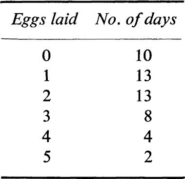
Show that this is approximately a Poisson distribution. Calculate the mean and standard deviation directly from the data. Compare with the standard deviation predicted by the Poisson distribution.
19. On the average, how many times must a die be thrown until one gets a 6 ?
HINT: Use the binomial distribution.
20. When 100 coins are tossed, what is the probability that exactly 50 are heads ?
HINT: Use the binomial distribution.
21. A bread salesman sells on the average 20 cakes on a round of his route. What is the probability that he sells an even number of cakes ?
HINT: Assume the Poisson distribution.
22. How thick should a coin be to have a i chance of landing on an edge.
HINT: In order to get an approximate solution to this problem, one may imagine the coin inscribed inside a sphere, where the center of the coin is the center of the sphere. The coin may be regarded as a right circular cylinder. A random point on the surface of the sphere is now chosen; if the radius from that point to the center strikes the edge, the coin is said to have fallen on an edge.
23. If a stick is broken into two at random, what is the average length of the smaller piece ?
24. Shuffle an ordinary deck of 52 playing cards containing four aces and then turn up cards from the top until the first ace appears. On the average, how many cards are required to produce the first ace ?
25. If n grains of wheat are scattered in a haphazard manner over a surface of S units of area, show that the probability that A units of area will contain R grains of wheat is

HINT : ndS/S represents the infinitely small probability that the small space dS contains a grain of wheat. If the selected space be A units of area, we may suppose each dS to be a trial; the number of trials will therefore be A/dS. Hence we must substitute An/S for np in the Poisson distribution P = (np)r e–np/r!
26. A basketball player succeeds in making a basket three tries out of four. How many times must he try for a basket in order to have probability greater than 0.99 of making at least one basket ?
27. An unpopular instructor who grades “on the curve” computes the mean and standard deviation of the grades in his class, and then he assumes a normal or gaussian distribution with this μ and σ He then sets borderlines between the grades at C from μ –The peak of the graph of the Poisson distribution ; σ /2 to μ + σ /2, B from μ + σ /2 to μ + 3 σ 12, A from μ + 3 σ /2 up. Find the percentages of the students receiving the various grades. Where should the borderlines be set to give the following percentages: A and F, 10 percent; B and D, 20 percent; C, 40 percent ?
28. A popular lady receives an average of four telephone calls a day. What is the probability that on a given day she will receive no telephone calls ? Just one call ? Exactly four calls ?
29. The Poisson distribution is used mainly for small values of μ = np. For large values of μ, the Poisson distribution (as well as the binomial) is fairly well approximated by the normal or gaussian distribution. Show that

The peak of the graph of the Poisson distribution is at x = μ; note that the approximating normal curve is shifted to have its center at x = μ. The equation given above gives a good approximation in the central region (around x = iμ) where the probability is large.
1939. von Mises, Richard: “Probability, Statistics and Truth,” The Macmillan Company, New York.
1955. Cramer, Harald: “The Elements of Probability Theory,” John Wiley & Sons, Inc., New York.
1957. Feller, William: “An Introduction to Probability Theory and Its Applications,”2d ed., vol. I, John Wiley & Sons, Inc., New York.
1960. Parzen, E.: “Modern Probability Theory and Its Applications,” John Wiley & Sons, Inc., New York.
1963. Levy, H., and Roth, L.: “Elements of Probability,” Oxford University Press, London.
1965 Fry, C. T.: “Probability and Its Engineering Uses,” 2d ed., D. Van Nostrand Company, Inc., New York.
1966 Feller, William: “An Introduction to Probability Theory and Its Applications,” vol. II, John Wiley & Sons, Inc., New York.
† See R. Courant, “Differential and Integral Calculus,” 2d ed., vol. I, pp. 361–364, Inter-science Publishers, Inc., New York, 1938.
† See Harald Cramer, “The Elements of Probability Theory,” pp. 97–101, John Wiley & Sons, Inc., New York, 1955.
† Paris, 1892.