In applied mathematics the need frequently arises for solving numerically transcendental or higher-degree algebraic equations; for example, in determining the natural frequencies of oscillation of a uniform prismatic bar built in at one end and with the other end supported, it is necessary to solve the transcendental equation
Transcendental equations occur very frequently in determining the natural frequencies and modes of oscillation of electrical and mechanical systems. Higher-degree polynomial equations also arise frequently in practice. Algebraic formulas exist for the solution of the general quadratic, cubic, and quartic equations with literal coefficients. However, no formulas exist for the solution of a general algebraic equation with literal coefficients if it is of higher degree than the fourth. The formulas for the cubic and quartic equations are sometimes laborious to apply to given cases. The importance of being able to solve numerically equations of this type is very great, and this appendix will be devoted to a brief discussion of possible methods of solution.
As an example, let us solve the transcendental equation
This equation occurs in determining the natural frequencies of oscillation of a clamped cantilever beam.
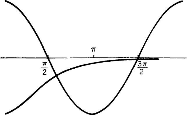
Equation (2.1) is satisfied by an infinite number of values of x. Let us write Eq. (2.1) in the form
If we plot the curves
and
the roots of (2.1) are given by the abscissas of the points of intersection of these two curves as shown in Fig. 2.1.
From the figure, we find the first three roots to be approximately
Since
the higher roots are given with satisfactory accuracy by the equation
Fig. 2.1
This example illustrates the general principle involved in the graphical solution of transcendental equations. That is, if we wish to solve the equation
we write it in the form
This may usually be done in many ways. We then draw the curves
The real roots of F(x) = 0 are evidently the abscissas of the points of intersection of these curves. The larger the scale of the graph and the more carefully the drawing is performed, the greater the accuracy of the roots. Having once found the approximate location of the roots, the accuracy may be improved by an iterative process called the Newton-Raphson method.
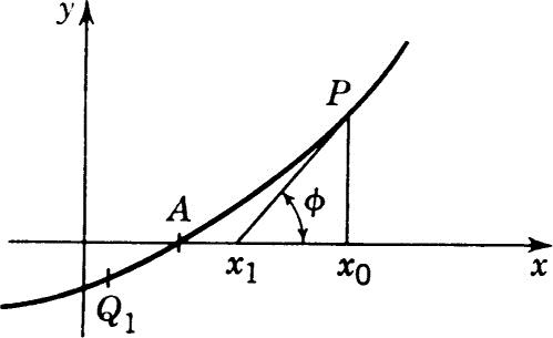
Let us consider the function
Let us draw this curve as in Fig. 3.1. The point x = A is a root of the equation
Let us draw the tangent to the curve at the point P. This tangent will intersect the x axis at a point x1.
From the figure we have
Hence
Fig. 3.1
it is apparent from the figure that this sequence tends to the root A. If we start on the other side of A where the arc of the curve is convex to the x axis, the first step carries us to the opposite side of A where the arc is concave to the x axis; after this the sequence tends to the root as before.
This discussion is based on the following two assumptions:
1. That the slope of the curve does not become zero along the arc Q1, P.
2. That the curve has no inflection point along Q1, P.
More precisely, we can say that, if F(x) has only one root between two points Q1 and P while F′(x) and Fʺ(x) are never zero between these two points, then the Newton-Raphson process will succeed if we begin it at one of the points for which F′(x) and Fʺ(x) have the same sign.
It is sometimes more convenient to use the formula
instead of (3.5).
This means that in the successive steps of the process we replace the tangents calculated at x1, x2, etc., by lines parallel to the tangent at P. This saves the trouble of calculating F′(xr) at each stage.
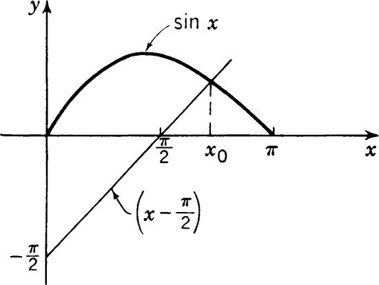
As an example of the method, let it be required to determine the solution of the equation
To obtain a rough estimate of the root, we draw the curves
as in Fig. 3.2.
Fig. 3.2
as a rough estimate of the root. With this value for x0, we begin the iterative process. Here we have
The first approximation is
Now
Hence
This is a very good approximation to the root. If more significant figures are desired, the iterative process of (3.6) may be repeated.
In the study of the natural frequencies of undamped electrical and mechanical systems with three degrees of freedom, we have to determine the solution of the equation
We may eliminate the Z2 term by the substitution
We then obtain
This may be written in the form
There are two principal cases to consider.
In this case the cubic has one real root and two complex roots. Then, if q and r are both positive, we find ϕ such that
Then the real root is given by the equation
Dividing (4.4) by x – x0, we reduce the equation to a quadratic and obtain the pair of complex roots by solving the resulting quadratic.
If q is negative and r is positive, we find ϕ such that
Then the real root is given by the equation
It may be noted that we may always suppose that r is positive since if we change the sign of r we merely change the sign of the roots.
b THE CASE WHERE 27r2 < 4q3
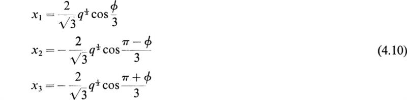
In this case the cubic equation has three real roots. We now find the smallest positive angle ϕ such that
Then the real roots are given by
For example, let it be required to solve
In this case we remove the Z2 term by writing
We now have
Hence this equation comes under case b, and the roots are all real. We now compute
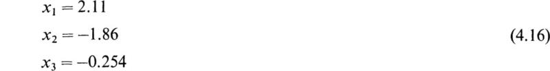
and, substituting into (4.10), we obtain
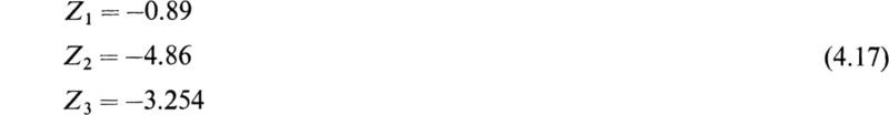
Hence the roots of (4.11) are
In the last section we considered some algebraic formulas for the solution of the cubic equation. There also exists a formula solution for the quartic equation.† These formulas are, in general, laborious to use in numerical computations. No formulas exist for the solution of a general algebraic equation with literal coefficients if it is of higher degree than the fourth.
In this section we shall discuss a method for the numerical solution of an algebraic equation of any degree. Before considering this method, it is well to recall the following properties concerning the nature of algebraic equations:
1. The equation
where the coefficients ar are real numbers, has exactly n roots. Some of the roots may be repeated roots.
2. If n is a positive odd integer, the equation always has one real root.
3. The number of positive roots either is equal to the number of variations of signs of the a’s or is less than this number of variations by an even integer (Descartes’ rule of signs).
4. The complex roots occur in conjugate complex pairs.
The method we shall consider was suggested by Dandelin in 1826 and independently by Graeffe in 1837. It is of great use, especially in the case of equations possessing complex roots. The fundamental principle of the method is to form a new equation whose roots are some high power of the roots of the given equation. That is, if the roots of the original equation are ![]() the roots of the new equation are x1, x2, . . . , xn., If s is large, then the high powers of the roots will be widely separated. If the roots are very widely separated, they may be obtained by a simple process.
the roots of the new equation are x1, x2, . . . , xn., If s is large, then the high powers of the roots will be widely separated. If the roots are very widely separated, they may be obtained by a simple process.
Let the roots of Eq. (5.1) be – r1, – r2, . . . , – rn. These values are the roots of the equation with the signs reversed and are called the Encke roots. (We shall assume at present that they are real and unequal.) Since the r quantities are the roots of the equation with the signs reversed, it may be factored in the form
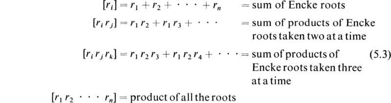
If we use the convenient notation
then on multiplying the various factors of (5.2), we obtain
A simple device by which one may obtain a new equation whose Encke roots are the squares of the Encke roots of the original equation will now be explained. Let us write
Then
and
If in (5.7) we let
we obtain
Now the roots of (5.9) are ![]() and hence the Encke roots are
and hence the Encke roots are ![]() and hence they are the squares of the Encke roots of (5.5). If we now write F(x) in the form
and hence they are the squares of the Encke roots of (5.5). If we now write F(x) in the form
then
Carrying out the multiplication and writing
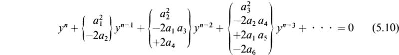
we obtain
This may be written in the form
We notice the coefficients of (5.9a) are found from the coefficients of the original equation (5.6a) by the following simple rule:
The coefficient of any power of y is formed by adding to the square of the corresponding coefficient in the original equation the doubled product of every pair of coefficients which stand equally far from it on either side. These products are taken with signs alternately negative and positive.
If a power of x is absent, then it is taken with a coefficient equal to zero. To facilitate the process, a table is constructed in the following manner:
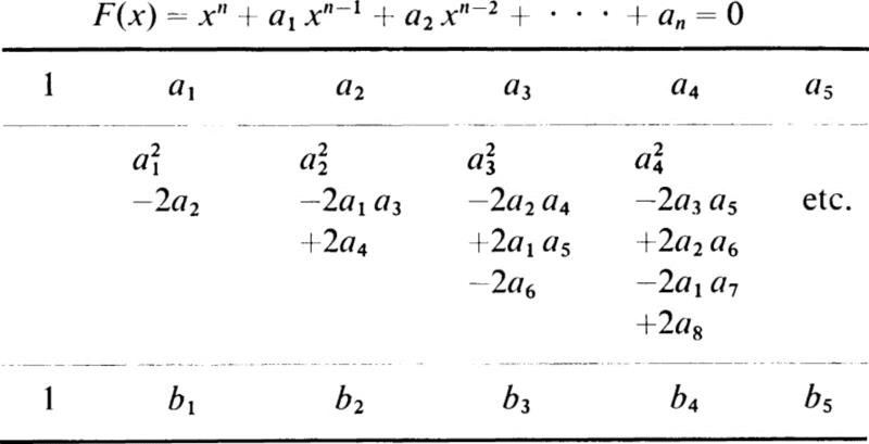
The b’s are the coefficients of the equation whose Encke roots are the squares of the Encke roots of the original equation.
If we now repeat this process several times, we finally arrive at an equation whose Encke roots are the mth powers of the Encke roots of the original equation. This equation has the form
If now
then
That is, if the roots differ in magnitude in the manner (5.12), then the mth powers of the roots, where m is a large number, are widely separated. Hence
for a sufficiently large m. We also have
Hence from (5.14) we obtain
and from (5.15) we have
Equation (5.16) determines the absolute value of the largest root r1, and Eq. (5.17) determines the absolute value of the second largest root r2, and so on.
In the solution of equations by this method it is very necessary to know when to stop the root-squaring process. The time to stop is when another doubling of m produces new coefficients ![]() that are practically the squares of the corresponding coefficients
that are practically the squares of the corresponding coefficients ![]() in the equation already obtained. To illustrate the general theory, let us consider the solution of the equation
in the equation already obtained. To illustrate the general theory, let us consider the solution of the equation
which has three real roots.
We construct the following table:
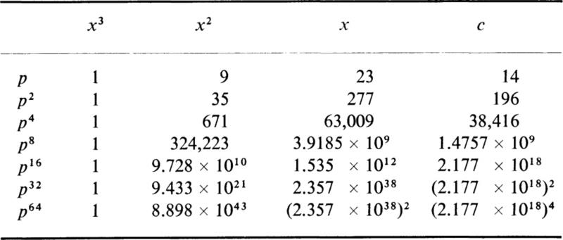
In this table p2 denotes the equation whose Encke roots are the squares of the Encke roots of p, etc.
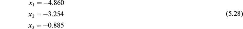
If we stop at this stage, we have
and hence
This is the magnitude of the numerically greatest root. We also have
Hence
Therefore
Finally, we have
and
and therefore
It is not possible to determine the signs of the roots by this process. Descartes’ rule of signs shows that all the roots are negative, and they are therefore
We shall now discuss briefly the modifications which must be introduced in the above procedure in case the equation under consideration has complex roots. To illustrate the general procedure, let the equation under consideration be of the fifth degree, and let it have the following Encke roots:
![]()
where
We carry out the root-squaring process as before and obtain an equation whose Encke roots are the mth powers of the Encke roots of the original equation. For a sufficiently large m we have
as before, since by hypothesis r1 is the dominant root numerically. Hence this root may be determined as before. We now have
If we let
we then have
This shows that the coefficient of the x3 term will fluctuate in sign as the number m takes in succession a set of increasing values because of the cosine term. We also have
Proceeding in this manner, we see that when m is large enough so that only the dominant part of the coefficient of each power of x is retained the equation whose Encke roots are the mth powers of the roots of the original equation is
From this we may find r1, r2, r3, and R. To obtain the angle of the complex root, we write
But we know that the sum of the Encke roots of the original equation is given by
Hence
or
In the above example we saw that the fluctuation of the coefficient of the x3 term indicated the presence of a pair of complex roots. If two coefficients fluctuate in sign, the presence of two pairs of complex roots may be inferred and the analysis modified accordingly. Rather than consider any fixed rules, it is well to consider the general nature of the root-squaring process in solving equations by this method.
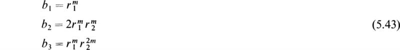
The nature of the process in case the equation has repeated roots may be illustrated by the consideration of a special case. As before, let the Encke roots of the equation be denoted by r1, r2, r3, . . . , rm. Let the root r2 be equal to the root r3,
That is, the equation has the repeated root r2. In this case again the equation whose Encke roots are the mth powers of those of the given equation is
If m is sufficiently large so that we may retain only the dominant term in each coefficient, we have
We notice that the coefficient of the term xn–2 does not follow the usual law that when m is doubled the coefficient is approximately squared. In this case, when m is doubled, the new coefficient is approximately half the square of the old one. This is an indication of a repeated root. To compute r2, let
If we divide b3 by b1, we obtain
and hence
The rest of the roots are computed as before. The foregoing discussion is the general theory of Graeffe’s root-squaring method. In general, it is better to keep the basic concept of the method of root squaring in mind rather than to formulate elaborate rules for special cases.
1. Determine the roots of the equation tanh x = tan x.
2. Determine the roots of the equation tan x = x.
3. Find the roots of ex = 5x.
4. Solve the equation x3 – 2x – 1 = 0.
5. Solve the equation x3 – 97 x – 202 = 0.
6. By using Graeffe’s method, solve the equation x2 – 2x + 2 = 0.
7. Solve the equation x3 + x2 + x + 1 = 0.
8. Find the roots of the equation x3 – 5x2 + 6x – 1 = 0:
(a) By the formula for the solution of a cubic equation.
(b) By Graeffe’s method.
9. Solve tan x = 10/x.
10. The equation x3 – 2x – 5 = 0 has a real root between 2 and 3. Determine the magnitude of this root by the use of the Newton-Raphson method.
11. Compute to four decimal places the real root of the equation x2 + 4 sin x = 0 by the use of the Newton-Raphson method.
12. Determine the roots of the equation x tan x = 10 to three decimal places.
13. Find the smallest positive root of the equation xx + 2x = 6 to three decimal places.
1918. Burnside, R., and F. Panton: “Theory of Equations,” 8th ed., vol. 1, Hodges & Figgis & Co., Dublin.
1924. Whittaker, E. T., and G. Robinson: “The Calculus of Observations,” Blackie & Son, Ltd., Glasgow.
1934. Cowley, W. L.: “Advanced Practical Mathematics,” Pitman Publishing Corporation, New York.
1936. Doherty, R. E., and G. Keller: “Mathematics of Modern Engineering,” John Wiley & Sons, Inc., New York.
1949. Milne, W. E.: “Numerical Calculus,” Princeton University Press, Princeton, N.J.
1950. Scarborough, J. B.: “Numerical Mathematical Analysis,” Oxford University Press, New York.
1952. Hartree, D. R.: “Numerical Analysis,” Oxford University Press, New York.
1954. Soroka, W. W.: “Analog Methods in Computation and Simulation,” McGraw-Hill Book Company, New York.
† See, for example, E. R. Dickson, “Elementary Theory of Equations,” p. 31, John Wiley & Sons, Inc., New York, 1922.