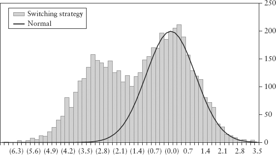
FIGURE 12.1 Bimodal Distribution of a Switching Strategy
The idea of reflexivity1 and its connection to market crashes and systemic risks has been studied and even published since 1987. Ironically, two decades and three crises have passed, and we still lack the tools to measure and safeguard our financial system from such a danger. Until very recently, most research was focused on phenomenology—explaining but not solving the problem. This chapter describes some key milestones in our understanding of the causes of systemic risk.
The salient feature of the current financial crisis is that it was not caused by some external shock like OPEC raising the price of oil or a particular country or financial institution defaulting. The crisis was generated by the financial system itself. This fact that the defect was inherent in the system contradicts the prevailing theory, which holds that financial markets tend toward equilibrium and that deviations from the equilibrium either occur in a random manner or are caused by some sudden external event to which markets have difficulty adjusting. . . . I propose an alternative paradigm that differs from the current one in two respects. First, financial markets do not reflect prevailing conditions accurately; they provide a picture that is always biased or distorted in one way or another. Second, the distorted views held by market participants and expressed in market prices can, under certain circumstances, affect the so-called fundamentals that market prices are supposed to reflect. This two-way circular connection between market prices and the underlying reality I call reflexivity.
—George Soros, Testimony during Senate Oversight Committee hearing, on the role played by hedge funds in the 2008 crisis
Soros first described the idea of market reflexivity in his book The Alchemy of Finance in 1987. His ideas ran against conventional economic theory that markets tend toward equilibrium as suggested by efficient market theory. Soros argued that the market is always biased in either direction (equilibrium is rare), and markets can influence the event they are supposed to anticipate in a circular, self-reinforcing way. This he termed reflexivity. However, this early reflexivity idea was couched in philosophy and behavioral science, not risk management.
Trading is decision making under uncertainty. Conventional risk modeling sees trading as a “single-person game against nature” where price uncertainty is driven by exogenous factors, and not impacted by the decision maker. This is frequentist thinking—an impartial observer scientifically taking measurements, inferring conclusions, and ultimately making decisions. This paradigm originates from the tradition of general equilibrium theory developed by Samuelson (1947), where macroeconomics is the aggregate behavior of a model where market participants or agents are rational optimizing individuals. Under this paradigm, statistical techniques can be used and indeed have been applied with great success, especially during normal market conditions.
However, during crises, conventional risk models break down. Market dynamics behave more like a game against other gamers—the drivers can be endogenous. Irrational herding behavior can occur without any external shocks. Prices can spiral out of control during a crash purely due to sentiment within the market. This could be caused by feedback loop effects between the actions of participants and outcomes, and spillover effect among participants within the system. Hence, after the 2008 crisis, there is a paradigm shift towards viewing the market as a complex adaptive system.
In the late 1990s, researchers began to formulate these effects in terms of game theory, Bayesian thinking, and network science. The network externalities (spillover) arise because each trader’s decision does not take into account the collective interest but ultimately affects it. For example, in a crash each participant hopes to beat the others to the exit. This risk of contagion increases with positional uniformity and leverage. It argues for the role of the regulator to intervene in free markets and to monitor for systemic risks on behalf of the collective interest.
Morris and Shin (1999) pointed out a blind spot in conventional risk management practice—value at risk (VaR) does not take into account the feedback loop between actions and outcomes. When many dominant players in the market follow a uniform strategy, the consequences of the feedback loop can be disastrous. For example, the 1987 crash was caused by portfolio insurance, a popular program trading strategy whereby institutions increase leverage in a rising market and deleverage in a falling market.2 The selling frenzy fed on itself on Black Monday. From 1997 to 1998, the Asian crisis was caused by concerted currency attacks by speculators, while local governments defended their currency pegs. Here, key players were amassing highly uniform positions.
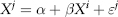
The authors proved that when a collective strategy is dominant, the usual bell-shaped return distribution can become distorted. Using the yen carry unwind in October 1998 as an example of a switching strategy,3 the return distribution was shown to be bimodal (has two peaks!). Hence, VaR will completely underestimate the true risk. If you plot the empirical distribution during that turbulent period, you will not see any evidence of bimodality. This is because the bimodal behavior happens only during the brief period of panic selling, too short to be captured by statistics. We can, however, simulate this behavior (see Spreadsheet 12.1). Figure 12.1 illustrates the bimodal distribution of a switching strategy where speculators have a stop-loss exit strategy slightly below the current level.
FIGURE 12.1 Bimodal Distribution of a Switching Strategy
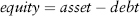
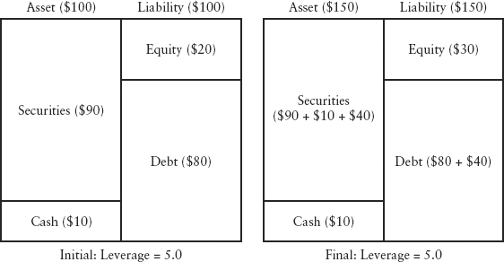
Adrian and Shin (2008) analyzed the role of feedback loops in exacerbating the 2008 crisis. The key idea is that leverage targeting by banks gives rise to procyclicality in the system, which accelerates the boom-bust cycle. Consider a stylized bank’s balance sheet presented in Figure 12.2. Assets and liabilities are always balanced; the balancing variable is the (shareholder’s) equity. Hence:
FIGURE 12.2 A Stylized Bank’s Balance Sheet Illustration
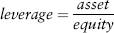
and we define:
In the left panel, leverage is 5(= 100/20) times. Suppose the price of (risky) securities goes up by $10, assets will increase to $110 by mark-to-market accounting, and leverage will fall to 3.67(= 110/30). In other words, asset growth and leverage growth should be inversely correlated if there is no change in positions. Surprisingly, empirical evidence by the authors showed that asset growth and leverage growth are highly positively correlated across U.S. financial institutions as a cohort. This suggests that banks actively manage their positions to maintain some target leverage.
Hence, leverage is procyclical, and that in turn can cause perverse asset price behavior. Consider the right panel; in order to maintain its initial leverage of 5 (suppose this is the target), the bank will borrow $40 more in debt to buy more securities that will bring assets to $150. Contrary to textbook norm,4 the demand curve for the asset becomes upward-sloping. The greater demand for the asset will put upward pressure on prices, and the price rally will lead to a stronger balance sheet, which necessitates even more purchases of assets to maintain the leverage target. Demand generates more demand in a self-reinforcing loop, and this can cause an asset price boom as shown in Figure 12.3 (left panel).
FIGURE 12.3 Asset Price Boom and Bust Caused by Procyclicality of Leverage
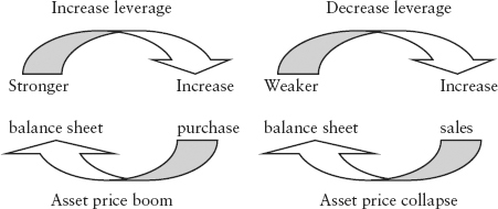
In an economic downturn, the mechanism works in reverse (right panel). Falling asset prices cause losses to the balance sheet, and leverage as defined in equation (12.2) increases. This will prompt banks to deleverage to maintain the target by selling off assets to pay off debt. The selling into a falling market can cause a downward price spiral and a sudden increase in supply (more people wanting to sell)—the supply curve becomes downward-sloping. This is called the loss spiral.
Another negative feedback is the margin spiral. Regulators require a minimum amount of capital to be set aside as a safety buffer (like a trading margin) usually determined by VaR. This can be represented simplistically as the cash portion on the asset side in Figure 12.2. The problem is that VaR is low during a boom and high during a downturn (see Chapter 7). Therefore, the same amount of cash margin can support a lot more risky securities during a boom than during a downturn—encouraging leverage during a boom and loss-cutting during a bust.
The Geneva Report (2009)5 identified key systemic risk drivers and negative feedback loops that contributed to the 2008 crisis; policy recommendations to address systemic risks were also discussed.
Contagion from participants during stressful market conditions is the root cause of the phenomena studied in Chapter 7. Positive feedback inadvertently causes serial correlation of returns that breaks the independent and identically distributed (i.i.d.) assumption and leads to volatility clustering. Stochastic volatility fattens the tails of the distribution. At the portfolio level, the distribution will become fatter than normal (leptokurtic) because the Central Limit Theorem (CLT) (which hinges on i.i.d.) no longer works. VaR becomes understated as the regime shifts to a more volatile state. There will be no pre-warning, after all, the sample distribution still contains mostly old data from a regular state. By this mechanism, the effectiveness of VaR becomes severely compromised during a crisis.
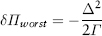
CrashMetrics was developed by Hua and Wilmott in 1998. Its purpose is to locate and estimate the worst-case scenario loss for a bank as a firm. The idea is that, since crashes cannot be delta-hedged in a continuous manner, especially with the presence of nonlinear derivatives, it makes sense to ask what is the worst loss for a bank given its positions. If a bank knows that this loss can threaten its survival, then it can static hedge6 this vulnerability. The static hedging with derivatives can be optimized to make the worst-case loss as small as possible. This is called Platinum Hedging (not covered here) and is proprietary to CrashMetrics.
Unlike VaR, CrashMetrics does not make any assumptions on return distributions. There are also no prior assumptions on the probability, size, and timing of crashes. The only assumption made is that crashes will fall in certain ranges (say from +100% to −50% price change).
Let’s consider a portfolio of derivatives on a single underlying asset. If the asset price changes by δS, the portfolio value π will change by:
where F(.) represents the sum of all pricing functions of the derivatives. So if it is an option, F(.) is the Black-Scholes equation; if it is a bond, F(.) is the bond pricing formula, and so on.
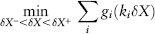
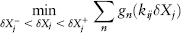
We need to find the worst-loss for the portfolio; that is, the minima for F(δS). In practice, to perform this minimization we need to constrain the domain of δS to within a finite range [δS−, δS+]. The risk controller just needs to assume a large but realistic range. The minimization problem then becomes:
For complicated portfolios, it is possible to have local and global minimas (to be explained later). We are interested in finding δS, which gives the global minima.
If the portfolio contains a vanilla option, F(.) will be a continuous function, and we can approximate δπ using a Taylor expansion:
where Δ and γ are the delta and gamma as defined in Section 4.1. The worst-case loss can be found by making the first derivative δπ/δS =0, which leads to the result:
Although this example is unrealistic (most banks would trade in nonvanilla options), it illustrates the procedure. Geometrically speaking, the minimization procedure involves searching the whole solution profile of δπ to find the lowest trough7 with slope δπ/δS = 0. For two assets, the profile is a surface; for N assets, the profile is an N-dimensional hypercube.
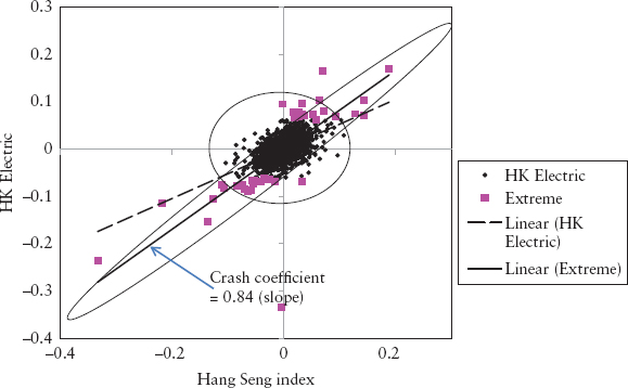
To extend the model to multiasset, we need to relate the extreme moves of each asset to the extreme moves of one (or more) benchmark index. For example, we can map all U.S. stocks to the S&P 500 index. The benchmark mapping is necessary to reduce the dimension to a manageable size. If the benchmark moves by X%, then the ith asset moves by kiX%, where ki is the crash coefficient for asset i. The crash coefficient is estimated using the beta approach (see equation (2.37)) except that we only use the 40 largest (extreme tail) daily moves in the history for asset i.
Figure 12.4 shows a scatter plot for HK Electric’s stock price returns versus its benchmark, the Hang Seng index, using the last 25 years of data. The circle and the oval show two distinct return regimes—normal and extreme. The slope of the (dotted) regression line for the full data set is the beta, whereas the slope of the extreme data set (line with higher slope) gives the crash coefficient, k = 0.84. Because of its shape, the diagram is called the Saturn ring effect. The crash coefficient is higher compared to the beta because assets are expected to be highly correlated during a crash. Furthermore, the crash coefficient is found to be more stable than the beta, which makes this method more robust.
FIGURE 12.4 Saturn Ring Effect Showing Different Return Regimes
With the presence of exotic options, the delta-gamma approach will not work, and a bank will need to do repricing of each deal in finding the worst-loss. For a multiasset/single index model, the minimization problem then becomes:
where δX is the change in the index, constrained to a finite range [δX−, δX+]. The sum is across i assets, all benchmarked to the same index; gi(.) is the pricing function for asset i.
The idea can be extended to multirisk factor where each factor is mapped to a benchmark. For example, we can have benchmarks for equities, rates, volatility, foreign exchange, and commodities. A deal may be mapped to one or more benchmarks. For example, an equity option can be mapped to an equity index benchmark and a volatility benchmark (such as the VIX index). Suppose there are i risk factors and j benchmarks (j < i), then the minimization problem becomes:
where the crash coefficient kij is the sensitivity of risk factor-i to an extreme move in benchmark-j. We need to solve for the set {δX1, δX2, . . . , δXj}, where each element (a benchmark) is constrained by a user-defined range, such that the overall portfolio value is the lowest. Note, the summation is across n number of deals, where the pricing function of a deal gn(.) can be a function of multiple risk factors generally.
It is possible to program an optimization algorithm to locate the global minimum in an N-dimensional hypercube efficiently and to compute the relevant hedge ratios (the so-called Platinum hedges). This is a sophisticated exercise and is proprietary to CrashMetrics. Here we will illustrate using a simple brute force implementation, which can be used as a bank’s stress/scenario testing to supplement VaR. The advantage is that while conventional scenario testing points to the risk of some hypothetical made-up situations, which could be unrealistic, CrashMetrics points objectively to a bank’s individual vulnerabilities. This should be appealing to regulators who can then compare worst-case losses among banks.
We first map the universe of all risk factors to five benchmark indices as shown in Table 12.1. The crash coefficient (ki) for risk factor i is estimated with respect to its benchmark index. When the benchmark index is stressed by δX, that risk factor is stressed by kiδX. In effect, the crash coefficients link risk factors to benchmarks. Hence, by stressing all five benchmarks, we effectively stress all risk factors.
TABLE 12.1 Mapping of Risk Factors to CrashMetrics Benchmarks
| Risk Factor Class (across all countries) | CrashMetrics Benchmark |
| Equities | S&P 500 index |
| Interest rates | USD 10-year swap |
| Foreign exchange rate | U.S. dollar index (measures dollar strength relative to a basket of currencies) |
| Volatilities (all asset types) | VIX index (measures implied volatility) |
| Commodities | S&P Goldman Sachs commodity index |
Secondly, we grid the hypercube. Suppose we have a small bank whose core business is in rates, FX, and options trading; thus, we only need three benchmarks. Suppose today’s state of the world is given by: (USD 10yr swap, U.S. dollar index, VIX index) = (3%, 78, 27%). We assume a range where the extreme moves can happen for each benchmark, for example: (USD 10yr swap, U.S. dollar index, VIX index) = (0 − 10%, 50 − 100, 2 − 70%), and grid each range into 20 equal segments. Then the hypercube will contain 20×20×20 = 8,000 states (or scenarios).
Thirdly, we perform reverse stress tests. The bank determines the maximum loss ψ that will cause it to fail. This critical level of loss is a function of the bank’s own balance sheet strength and its ability to raise emergency funds. The bank’s positions are repriced for all scenarios in the hypercube. The scenarios that create a loss larger than ψ are highlighted as red zones in the hypercube.
Lastly, expert judgment is required of the risk controller. What is the probability of occurrence of the red zones? This is a function of how far they are from the current state and known structural relationships of the markets. It requires expert knowledge of probability and correlation. For example, if a red zone happens when rates are at 10%, the odds are really immaterial for say a one-year risk horizon. Is it likely for rates to move from 3% to 10% in a recessionary, low policy-rate environment? Also if the red zone suggests a scenario of extreme sell-down in equities and extremely high rates, this is also highly unlikely (perhaps even unrealistic) because equities and rates are known to be structurally correlated due to fund flows, flight-to-quality, and central bank policy responses.
This brute force method illustrates a rough way to locate a bank’s vulnerabilities. The method is crude because errors can arise from the estimation of crash coefficients and the choice of benchmarking. It should always be followed by stress tests targeted at a bank’s specific vulnerabilities (or risk concentration).
As an example of the application of CrashMetrics, please refer to Gomez, Mendoza, and Zamudio (2012). A spreadsheet demo of CrashMetrics is downloadable from: http://thehedger.wikispaces.com/file/view/23.CrashMetrics.XLS.
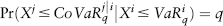
Contagion VaR or CoVaR was introduced by Adrian and Brunnermeier (2009) to measure the spillover risk across financial institutions. Specifically, it is defined as the VaR of institution i conditional on another institution j being in distress; that is, j’s return being at its VaR level.
CoVaR measures volatility spillover in a noncausal sense. The idea is that institutions often hold similar positions or are exposed to common systemic risk factors. These crowded trades give rise to dynamic competition games, which can cause liquidity spirals. For example, in an asset fire sale or banks’ hoarding of liquidity, individual actions by banks may appear prudent for the bank, but the impact on the system is often not macroprudential. CoVaR measures this spillover or network effect.
We recall the definition of VaR as the q-quantile:
where Xi is a variable of institution i, and VaR is a negative number. The time series Xi may be the daily profit and loss (PL) vector of the bank’s positions, or changes in the bank’s total financial assets in its balance sheet, depending on what type of spillover risk we want to measure.
The CoVaR of institution j conditional on institution i being in distress is then defined as:
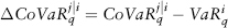
We are most interested in the case where j is the entire financial system (j = system). In this case, the institution i’s contribution of spillover to the financial system (j) is defined by:
Studying data on U.S. financial institutions, the authors found evidence of spillover—that CoVaR tends to be larger than VaR in general, making equation (12.11) positive. Furthermore, a linear regression of ΔCoVaR and VaR shows an absence of a linear relationship, which suggests that conventional VaR does not contain information on systemic risks at all: hence, the need for CoVaR.
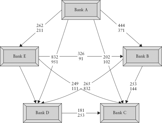
Figure 12.5 shows a schematic of CoVaR between various institutions. CoVaR of institution i depends on the risk-taking activities of other institutions in the network. CoVaR is also directional—CoVaR of institution i conditional on j does not equal CoVaR of institution j conditional on i in general. This is illustrated as two different numbers on each connecting line in Figure 12.5.
FIGURE 12.5 Schematic of CoVaR Network (Numbers Are Hypothetical)
The systemic risk regulator would in principle be able to collect all the required information Xi from each institution and calculate an institution’s contribution to systemic risk using equation (12.11). Regulatory risk capital should then be a function of not just VaR but also ΔCoVaR—large contributors to systemic risk should be surcharged with higher capital.
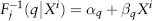
A convenient way to estimate CoVaR is by quantile regression (see Section 2.13). Here we assume j is the financial system and is related to bank i’s return variable by a linear model:8
where Xs are a function of time t (which we have suppressed for brevity), and the error term εj is i.i.d. We denote the inverse CDF by F−1(q) for a given q-quantile. Then the inverse CDF for (12.12) is written:
where the new parameters αq and βq contain also the inverse CDF of εj. From the definition of VaR as a quantile function or inverse CDF, equation (12.13) actually represents the VaR with confidence level (1 − q) of system j conditional on the returns of institution i.
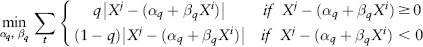
We estimate the conditional quantile function (12.13) by solving for the parameters αq and βq that minimize:
Since CoVaR is defined as the VaR of j conditional on bank i’s return being at its VaR level (i.e., set Xi = VaRiq), the CoVaR is thus given by:
The parameters with the ^ are estimates from (12.14). Spreadsheet 12.2 illustrates the calculation of CoVaR using the Excel Solver.
In the original paper, the idea of CoVaR was extended to make Xi, Xj, and equation (12.12) conditional on other lagged variables Mt−1. These could be systemic macro variables—such as the volatility index (VIX), repo spreads, T-bill yields—or a firm’s institutional characteristics—such as maturity mismatch, leverage, relative size, and so on. In particular, the authors found that, on a one-year lagged basis, a more negative δCoVaR is associated with higher values of the institutional characteristics just mentioned. The implication is that if regulators can predict, based on today’s firm characteristics, what the δCoVaR will be for next year, it can levy a preemptive capital surcharge. This means δCoVaR capital could potentially offset the procyclicality weakness of conventional VaR. For further details, the reader can refer to the paper by Adrian and Brunnermeier (2009).
In 2006, researchers at the Austrian Nationalbank (OeNB) introduced a model to measure the transmission of contagion risk in the banking system. Called Systemic Risk Monitor (SRM), it is based on the work of Elsinger, Lehar, and Summer (2006a, 2006b), which combines standard risk management techniques with a network model9 to capture the interbank feedback and potential domino effect of bank defaults. Only by looking at risk from the system perspective can regulators spot two key problem areas that could lead to financial system instability—correlated exposures and financial interlinkages.
This section gives a simplified illustration of a highly complex series of models. The interested reader is referred to the original papers.10 Figure 12.6 is a schematic of the SRM that was applied to the Austrian banking system. Each bank in the system is represented by a portfolio.
FIGURE 12.6 Basic Structure of the SRM
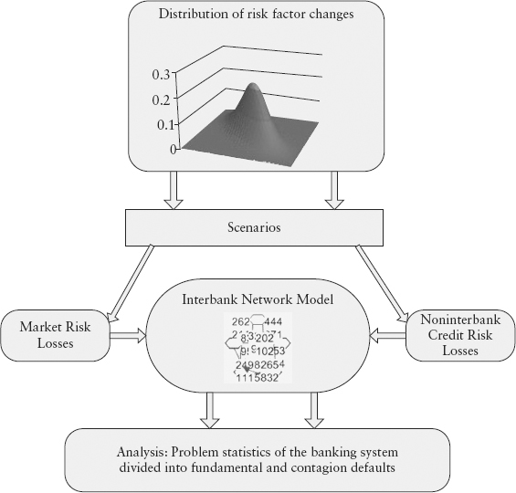
The model structure splits a bank’s risk into three parts—a collection of tradable assets: that is, stocks, bonds, forex (“market risk losses” box), loans to nonbanks (“noninterbank credit risk losses” box); and interbank positions (“interbank network model” box); and the third part captures the mutual obligations or counterparty risks, which are highly contagious.
The model uses a group of risk factors including market and macroeconomic factors. The (marginal) distribution of each factor is estimated separately every quarter for a one-quarter horizon. The correlation structure is modeled separately using a copula. The SRM model then draws random scenarios from this multivariate distribution (the top box in Figure 12.6). The scenarios are then translated to portfolio PL. For market risk losses, this is a straightforward revaluation of deals based on new scenarios. But for loans to nonbanks, we need to use a credit risk model to calculate portfolio losses. For this purpose, SRM uses CreditRisk+ developed11 by Credit Suisse in 1997.
The innovation of the Austrian model is its network model of the interbank, which checks whether a bank is able to fulfill its financial obligations as a result of simulated movements in asset prices and loans, given its balance sheet situation and mutual obligations with other banks. It does this by using a clearing procedure, which we shall illustrate using a toy example from the original paper by Elsinger and colleagues (2006a).
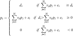
Suppose there are N banks in the system; bank i is characterized by net value ei and liability lij against bank j in the system. The entire banking system is thus described by an N × N matrix L and a vector of values e = {e1, e2, . . . , eN}. e represents asset positions such as bonds, stocks, and nonbank loans, minus liability positions such as deposits and bonds issued by the bank itself.
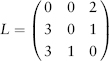
Consider a three-bank system with e = (1, 1, 1) and with liability structure given by:
where the numbers are in billions of dollars. For instance, bank 2 has a liability of $3 billion with bank 1 and a liability of $1 billion with bank 3. The diagonals are all $0 since a bank will not have a liability with itself. The total liabilities of each bank due to the system is given by the vector d = (2, 4, 4), the row sum of L. Note that the total income due from the system is given by the column sum of L.
The clearing mechanism is a redistribution scheme—if the net value of a bank becomes negative, the bank becomes insolvent. This net value is the income from noninterbank activities ei plus income received from other banks (part of L) minus its liabilities to other banks (part of L). Once a bank becomes insolvent, the claims of the creditor banks are satisfied proportionally; that is, distributed according to the percentage of total liability owed. To implement this proportion sharing, we need to divide L by d to get a normalized matrix in percentage:
In our example, this becomes:
The network model is represented by a clearing payment vector, p. The model has to respect the limited liability of banks (i.e., it cannot pay more than what it has in capital) and proportion sharing; pi represents the total payment made by bank i under a clearing mechanism.
The first condition says that the bank has enough income to pay off its total liability, and so it pays di due to the system. In the second condition, it pays proportionally as determined by weights πji, and in the third its payment is floored at zero due to limited liability. In the last two cases, because pi < di, bank i has defaulted with recovery rate pi/di.
To solve for the vector p, Eisenberg and Noe (2001) proposed a procedure called fictitious default algorithm and proved that the procedure converges to a unique solution after at most N iterations. The procedure starts by assuming all banks fully honor their obligations; that is, p = d. After this payment, if all banks have positive value the procedure stops. Second iteration: if a bank now has a negative value, it is declared insolvent, and its payment is given by the clearing formula, equation (12.19). In the example, this is the case for Bank 2. We keep the other bank’s payments fixed as per the previous iteration. It can happen that another bank that was positively valued in the first iteration becomes negatively valued (defaulted) in the second iteration because it only received partial payments from Bank 2. This is indeed what happened to Bank 3. Then Bank 3 has to be declared insolvent, and we move on to the third iteration and so forth.
A bank that becomes insolvent in the first iteration is considered fundamentally defaulted; that is, due to macroeconomic shocks. A bank that defaults in subsequent iterations is dragged into insolvency and represents a case of contagion default. Using the algorithm, we can show that the clearing solution is p = (2, 1.87, 3.47), Bank 2 is fundamentally defaulted, and Bank 3 experienced a contagion default. Spreadsheet 12.3 provides a worked-out solution.
In practice, L comes from balance sheet information of banks, and e is a function of risky positions held by banks—both of which are at the disposal of an ardent regulator. Market/economic scenarios sampled from the joint distribution are applied to e to simulate the risks caused by external shocks over a three-month horizon. Spreadsheet 12.3 also provides an example where e is randomly simulated to calculate the probabilities of fundamental and contagion defaults of the three banks.
The SRM system is a powerful tool that can simulate systemic risk conditions and identify vulnerabilities in a banking system. Some analyses that could be carried out include:
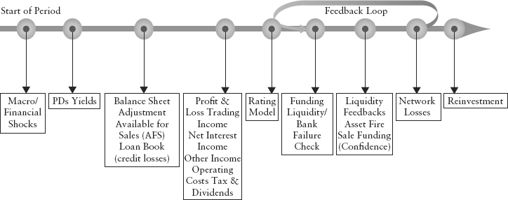
In 2009, the Bank of England (BOE) embarked on a project to model the network funding liquidity risk of the U.K. banking system. The model is a more sophisticated extension of the Austrian model and is known as RAMSI (Risk Assessment Model for Systemic Institutions). RAMSI is a sequence of models designed in a modular architecture (see Figure 12.7).
FIGURE 12.7 RAMSI Framework
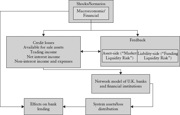
The innovation of RAMSI is in its modeling of feedback effects: the feedback associated with asset fire sales following a bank default and the liability-side funding liquidity feedback. Unlike the single-period Austrian model, RAMSI is a multistep model with a three-year forecast horizon (see Figure 12.8). A preliminary model description is available from the BOE.12
FIGURE 12.8 RAMSI Model Dynamics
The 2008 crisis has highlighted the complete absence of regulation of systemic risk. The Turner Review aptly described this situation as “global finance without global government: faultlines in regulatory approach.” National regulators do not have cross-jurisdiction powers, and coordination among regulators is not effective and timely. Even within the same country, supervision is often fragmented with multiple regulators looking at different but overlapping aspects of the financial system such as securities houses, futures trading, banking, insurance, and financial accounting. Quite the opposite, global banks operate across international borders, often exploiting differences in regulations so as to be as capital-efficient as possible, for example, by migrating operations to regulatory or tax-friendly jurisdictions.
There is asymmetry of information here: A bank knows exactly what its offshore branches are doing, but not what other banks are doing. An individual regulator knows only what the banks within its borders are doing and not about offshore banks. The informational disconnect creates a faultline where systemic risks can grow undetected by any one party.
Compounding the problem is that a new class of institutions (what is now known as shadow banking) has emerged that functions like a bank but is not regulated as a bank. These are entities such as SIVs (special investment vehicles), pure investment banks, and mutual funds, which perform the essential banking function of maturity transformation—effectively borrowing on short-term (liability), and lending or investing on long-term (asset). It is a crucial function that provides social and economic value, but it creates risks—there is price risk on the asset side and liquidity risk on the funding side. This large shadow banking system contributes to systemic risk (contagion) because their positions are often on the same side as regulated banks. In a crisis, they may face investor redemptions in the same way that a bank may face bank runs, even though they are off the radar screens of regulators, and are often too big to fail.
These faultlines argue for the creation of systemic risk regulators, of which three were set up in 2009: the Financial Stability Board (FSB), which represents the G-20 nations; the European Systemic Risk Board (ESRB) from the European Union; and the Financial Services Oversight Council (FSOC) from the United States. It seems logical that a single global regulator would solve some of the coordination problems previously mentioned and reduce political lobbying. But in the near term, this will unlikely materialize for the same reasons that one cannot find a global government today.
Let’s for the moment envision how such a regulatory body would work. It should have executive powers to investigate a bank13 (in a more intrusive way), technical expertise, political independence, and a modus operandi not unlike that of a tsunami warning center. Some of the technical roles it will perform may include:
Most of these ideas are within reach of today’s risk technology and knowledge. Basel III rules encourage over-the-counter derivatives to be processed and cleared with an independent third party, the central counterparty (CCP). This would set the stage for greater transparency and availability of data for a systemic regulator. The CCP will eliminate counterparty risk (in theory) since the CCP is effectively the counterparty to each trade and will maintain the usual margining safeguard. For a participating bank, a deal posted at the CCP will benefit from low capital requirement.
In the testimony to the U.S. House of Representative, Lo (2009) recommended the data collection and centralized monitoring of seven aspects of systemic risks: leverage, liquidity, correlation, concentration, sensitivities (to market movement), implicit guarantees, and connectedness. For a recent development in systemic risk measurement, read Billio and colleagues (2010).
1. We use this term generically to mean what many researchers also call feedback loop, vicious cycle, endogenous risk, and network externalities.
2. The program effectively tries to mimic the payoff of a call option so that the downside of the portfolio is protected. It does this by calculating all the correct sizes and levels to buy or sell. Execution is automated.
3. Hedge funds attacked the yen in 1998 while the central bank, BoJ, was hopelessly defending the yen. The tide turned after the Russian debt default (August 1998) and the LTCM debacle (September 1998) caused nervous speculators to abandon the attack. In this case, certain events or price levels caused the market (which held a uniform position) to switch strategy en masse. The rush-to-exit (unwind) caused the yen to rise by 15% in the week of October 5–9.
4. In classic economic theory, the typical demand curve (plot of Price versus Quantity) is negatively sloping, and the typical supply curve is positively sloping. The crossover of the two curves (on the Price versus Quantity plot) gives the equilibrium price where demand is satisfied by supply.
5. Brunnermeier, M., A. Crocket, A. Persaud, and H. S. Shin, “The Fundamental Principles of Financial Regulation,” Geneva Reports on the World Economy 11 (2009).
6. Dynamic hedging (or delta hedging) of a derivative involves continuously buying and selling the underlying asset of that derivative in such a way that the combination has a delta (and perhaps also other risk sensitivities) of zero at any point in time. A static hedge, in contrast, is not adjusted over time and is targeted to protect very specific vulnerabilities.
7. It can happen that, for a complicated portfolio, there may be multiple troughs in the solution space. The lowest trough is called the global minimum; all other troughs are local minima. A good optimization program is able to find the global minimum while avoiding all the local minima.
8. For ease of explanation, we illustrate a simplified version of the authors’ paper. In the original paper, Xj is conditional also on a vector of external state variables Mt-1, and the stochastic third term (hence volatility) is also conditional on Xi.
9. The network model is due to an earlier work by Eisenberg and Noe (2001).
10. For a nontechnical overview, please see “Systemic Risk Monitor: A model for systemic risk analysis and stress testing of banking systems,” OeNB Financial Stability Report 11.
11. This model (unlike Creditmetrics) models only default risk; migrational risk is excluded. The default risk is not related to the capital structure of the firm but is modeled simply as a Poisson distribution.
12. See BOE Working Paper No. 372, “Funding Liquidity Risk in a Quantitative Model of Systemic Stability” (June 2009).
13. We use the word bank generically to also include all other systemically important institutions (shadow banks).
14. For example, Oest and Rollbuhler, “Detection and Analysis of Correlation Clusters and Market Risk Concentration” by Wilmott Magazine (July 2010).