
Walrasian Equilibrium in the Case of a Single Labor Sector
1.Significance of the Quantity ρmax
We continue to develop the consequences of the definition of a price equilibrium. In the previous lecture we saw that condition (b)–the condition that each firm of the model optimize its own profit –implies the existence of a number p, the same for all firms, defined by
for all values of i = 1, · · ·, n. If these equations are written

we see that we have merely returned to the price theory of the third lecture. If, as in Lecture 3, we define the number ρmax to be dominant of the matrix πij with the j = 0 column removed, so that

the results established in the first four lectures show that ρmax is a certain number, which is a supremum of the set of numbers ρ for which (14.2) has a solution ρ with all pj ≥ 0. The number ρ we call, as previously, the rate of profit. We saw in these earlier lectures that (14.2) determines the price ratios as a function of p; we may consequently write pj(p), j = 0, · · ·, n, for the solution (unique up to a common factor depending on p) of the equations (14.2). The functions pj(ρ) are, of course, defined only for ρ ≤ ρmax.
If the number ρmax is negative, it therefore follows at once that ρ is negative. Hence, at equilibrium each firm must sustain a loss on every item it produces, so that the firm attains its maximum profit by producing nothing at all; all the production levels aj(k) are zero, and the case is devoid of interest. We will consequently confine our attention to cases in which ρ ≥ 0, and hence to cases in which ρmax ≥ 0 and to the range 0 ≤ ρ ≤ ρmax. Since we know from the results established in the first four lectures that if ρmax ≤ 0 then no arrangement of production levels can produce a nonzero surplus, we see that this restriction is not in the least unnatural.
It follows from the results established in Lecture 3 that pi(ρ) > 0 for 0 ≤ ρ ≤ ρmax and i = 1, · · ·, n, while po(ρ) > 0 for ρ ≤ ρ < pmax.
2.Necessary Conditions for Equilibrium
Let us now try to analyze the interesting case–that in which ρmax is positive. We assume the existence of a price equilibrium and develop the properties of such an equilibrium. Condition (b) implies, as was shown in the preceding lecture, that unless ρ = 0, every firm must utilize all its capital in production. Thus its profit must be exactly ρ times its total capital, i.e., 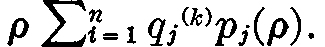 The profit of each firm is then evidently a function of ρ only, because the price ratios are functions of ρ only. Now since the profit of each firm is a function of ρ alone, and since the share in ownership of each firm held by each family is a given quantity, the dividend income of each consumption unit (family) is also a function of ρ alone. Accordingly, we may write the expression

for the dividend income of the vth family. If ρ = 0, this expression degenerates to zero, and thus remains correct.
The utility function u(v)(s0, · · ·, sn), (remember that s0 is negative while s1, · · ·, sn are positive) is assumed, in the manner explained in the preceding lecture, always to increase if a suitable one of its arguments is increased; therefore, in maximizing the u(v) subject to the budgetary condition (c), i.e., subject to the condition

equality is always attained, i.e., we always have

at the maximum of utility. (To maximize utility, all income from wages and dividends must be spent.)
If, as we shall henceforth assume, the maximizing [s0(v), . . ., sn(v)] is unique, it is then clear that from the preceding equation and from (14.4) that the quantities sj(v) depend only upon ρ; thus each family’s demand for commodities is a function of ρ alone. We will indicate this fact in what follows by writing these quantities as S0(v)(ρ), si(v)(ρ), . . ., sn(v)(ρ). (It is possible and even customary to introduce geometric conditions under which the above maximum will be unique, but they are rather artificial. Therefore we introduce uniqueness of the maximum explicitly as an additional assumption.)
Next we define

then si(ρ) is the total demand for commodity Ci, while S0(ρ) is the total amount of labor offered by all the families. As the notation suggests, the si(ρ) are functions of ρ alone.
Let  so that ai is the total amount of the commodity Ci produced. Since all of the prices, excepting possibly p0,, are positive, condition (d) yields

which determines the total production levels ai as a function of ρ. Moreover, again by condition (d), equation (14.7) holds for j = 0 as well, unless p0(ρ) = 0, i.e., unless ρ = ρmax.
Let d0(ρ) be the total demand for labor, i.e., let

Then for ρ < ρmax, equation (14.7) says

while if ρ = ρmax, condition (d) gives directly

We now have sufficiently many equations in hand. What do they mean? Let us review: we start with the fact that at equilibrium prices are determined competitively, and hence by the rate of profit ρ. From this we deduce that dividend income, hence consumption and total production levels, are all determined by ρ. All that remains is the determination of this one number ρ. This is determined as follows: the supply of labor is determined by ρ (through the utility functions). The demand for labor is also determined by ρ (through the utility functions and the demand for other commodities). Thus, unless ρ = ρmax, the rate of profit is determined by equation (14.9): demand = supply, for labor. This familiar conclusion remains banal unless we have some information on the form of the schedules of demand and supply for labor. We now turn to the elucidation of those schedules.
3.Supply and Demand of Labor
We first investigate the form of the function –s0(ρ). Unthinking economic habit might lead us to assume that –s0(ρ) must be a monotone decreasing function of ρ, since we may argue that labor, like any other commodity, is subject to the “law of supply,” which normally would require that as the wages paid to labor go down (as a result of increasing ρ) the amount of labor which people are willing to supply must also go down. The supply of labor is governed differently, however, as many authors have observed. When wages fall low enough, people must work more in order to get by; second members of families, women, children, etc., all enter the market in this range of wages; thus there is a minimum in the plot of s0(ρ) against ρ. This fact has been consciously used in determining the wage level in many parts of the world. If, however, wages fall to the point where the labor force can no longer subsist, then the labor offered must fall rapidly to zero. This “subsistence effect” would take place for a value of ρ close to ρmax. The qualitative form of the labor supply schedule, i.e., the graph of –s0(ρ) against ρ, must then be as shown in Fig. 19.
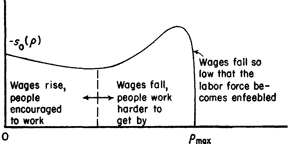
Fig. 19. Supply of labor plotted against the profit rate.
The demand d0(ρ) arises, as equation (14.8) shows, from the demand for commodities. This latter demand is generated, as equation (14.5a) shows, by income from two sources: by wage income and by dividend income. The demand for labor may therefore be approximately regarded as a sum of two terms: the demand for labor generated by wages and the demand for labor generated by dividends. The demand d(1) for labor generated by wages depends, of course, upon wages; it may be obtained approximately by multiplying the actual labor offered (for a given ρ) by the wage rate. Thus it has a nonzero value for ρ = 0, and falls to zero when ρ = ρmax If we multiply the schedule s0(ρ) in Fig. 19 by the wage rate, we will obtain a schedule which is qualitatively like the schedule drawn in Fig. 20; knowing little about its detailed form, we may still be confident that it is not grossly misrepresented by an approximately straight line. A plot of d(1)(ρ) against ρ, obtained by multiplying S0(ρ) by the wage rate is shown in Fig. 20. The demand d(2) for labor generated by dividends is, of course, to a good approximation a linear function of the rate of profit, since, at full utilization of capital, profits depend linearly on rate of profit. This is shown in Fig. 21. The total demand for labor d0(ρ) = d(1)(ρ) + d(2)(ρ) must then be quantitatively as shown in Fig. 22; though which of cases (a), (b), and (c) subsist, our rough arguments do not tell us.

Fig. 20. Demand for labor generated by wages as a function of the rate of profit.
Fig. 21. Dividend-generated demand for labor and rate of profit.

Fig. 22. Total demand for labor against rate of profit.
The rate of profit must now satisfy the relation

(unless ρ = ρmax). To see what this means, let us superimpose the curves of Fig. 19 and Fig. 22 in a single plot as shown in Figure 23.

Fig. 23. Supply and demand for labor. Three hypothetical cases.
(In drawing this figure, we have made use of the fact, to be established in the next lecture, that s0(0) = d0(0). We will show in the next lecture that in spite of this identity, ρ = 0 is an equilibrium point only if (d/dρ)(d0(ρ) + s0(ρ)) | ρ=0 > 0.)
Three cases arise, according to the slope of the curve of demand for labor. In case (a) the only solution for ρ is ρ = 0. This is the case in which an incorrigibly lazy populace refuses to work except to an amount so small that not all capital is utilized. In this case, ρ falls to zero and everything which is produced is turned back to the populace to be consumed. In case (b) people are “lazy” in this sense unless wages are sufficiently small. This means that, if wages rose from their equilibrium value, so many people would decide not to work, or decide to work only sporadically, that a labor shortage would develop. While this theoretical situation has often been taken as descriptive of the woes of management in establishing, say, rubber plantations among primitive populations not accustomed to regular industrial labor, it is hard to believe that it is descriptive of an economy like that of the United States. The United States, we must hence rather assume, falls into our case (c).1 We are then led inexorably by the present neoclassical theory to the unpalatable conclusion that the supply of labor exceeds the demand up to that point where wages are so low that the labor force becomes enfeebled.
Why is this not the case? To escape from our dilemma we must note that the demand for labor rises with its price: If the demand for labor fell as its price rose, we would necessarily be either in case (a) or in case (b) (cf. Fig. 23!). How can this apparently paradoxical behavior be understood? A full answer must await our subsequent development of a more general equilibrium model incorporating the Keynesian features which the present model neglects. Nevertheless we may give part of the answer without difficulty. There is in our model no substitute for labor, so that even ordinary supply-demand considerations would tell us that demand should be insensitive to price; whether demand for labor increases or decreases with its price, the present theory does not suggest. This fact is often missed, in consequence of the fact that equilibrium analysis is normally “partial” rather than “general.” Realizing this, we must next realize that such a situation—demand rising with or insensitive to price—is a ready-made temptation to monopoly (a similar remark may be made about any essential commodity, i.e., any commodity with price-inelastic demand). The role of trade unions is then quite clear. Unions have a product to sell for which the demand is much the same or even greater the higher the price. If, by one or another method, to be graphic, say by the hiring of thugs to murder anyone offering to work below a certain wage, the labor supply curve is made to fall to zero at that wage, then the aforesaid wage (and corresponding profit rate) will be the equilibrium.
The proper conclusion at this point is that the rate of profit ρ is not successfully determined by the Walrasian theories from consideration of production coefficients, utility functions, and so forth. What our analysis shows, in fact, is that the determination of the rate of profit is not purely a question of economics at all, but is rather a social-political question involving, among other things, union-management relations, pressures and counterpressures, etc. Thus an initial skepticism about classical equilibrium analysis is justified. What this analysis aims to give us is a set of prices. But all the price-ratios are already determined by a small part of the theory, to wit by the competitive equality of profit rates. All that remains to be determined on the score of prices, is the rate of profit—but, as we have just seen, the Walrasian determination of this rate is questionable. (If taken seriously, it justifies the most pessimistic views on the wage of labor, to which views there has been much objection!) What are determined more successfully are the amounts of production—but this is more a humble matter of consumption habits at given prices than a highly recondite matter of consumption schedules at a variety of hypothetical prices.
It is interesting to compare our conclusions with the views expressed by Mr. Henry Hazlitt in a passage which we have already cited once:
If I were put to it to name the most confused and fantastic chapter in the whole of the General Theory, the choice would be difficult. But I doubt that anyone could successfully challenge me if I named Chapter 19 on “Changes in Money-Wages.”
Its badness is after all not surprising. For it is here that Keynes sets out to challenge and deny what has become in the last two centuries the most strongly established principle in economics—to wit, that if the price of any commodity or service is kept too high, (i.e., above the point of equilibrium) some of that commodity or service will remain unsold. This is true of eggs, cheese, cotton, Cadillacs, or labor. When wage rates are too high there will be unemployment. Reducing the myriad wage rates to their respective equilibrium points may not in itself be a sufficient step to the restoration of full employment (for there are other possible disequilibriums to be considered), but it is an absolutely necessary step.
This is the elementary and inescapable truth that Keynes, with an incredible display of sophistry, irrelevance, and complicated obfuscation, tries to refute.
1 This implies that the demand for labor schedule slopes downward with increasing ρ, cf. Fig. 23. This empirical conclusion corresponds to the fact, to be emphasized below in our discussion of the propensity to consume, that the transfer of income from the low-income to the high-income range reduces total consumption. Of course, as was pointed out in the previous lecture, the present Walrasian and the Keynesian models which lead to such conclusions are not entirely comparable.