The previous chapter exploited a tiny data set of only a half-dozen observations. The prices in these observations appeared to be market prices, and I treated them as such. There was, however, no demonstration that they were market prices, that is, that they were the results of changing supplies and demands as explained in chapter 1.
One reason it has been hard to demonstrate the existence of ancient markets is that there is a paucity of ancient prices in the surviving records. Duncan-Jones (1982) and Rathbone (1997) collected prices for common articles in an agricultural economy—albeit one with many monuments and statues. Even though they found a large number of prices, the prices were spread over many commodities and even more years. One has only to look at the small number of observations found by these authors to realize that only the simplest of hypotheses can be tested. Hopkins (1978, 158) reported what he called “the largest single series of prices over time which we have from the classical world.” The series contained seven hundred prices that slaves paid for their freedom, spread over the last two hundred years before the Common Era. Slaves, of course, were very diverse, and there were far fewer observations for any subsets of more similar slaves. He observed a rise in release prices over these years but could not test complex hypotheses.
In this context, Slotsky’s (1997) report of what appeared to be a series of monthly market prices for six agricultural commodities for four hundred years in Hellenistic Babylon appeared to provide much more evidence of ancient market activity than had been available earlier. But although Slotsky argued that her observations were market prices, her interests were primarily historical and philological rather than economic. This chapter pursues the economics of these observations to answer two questions. First, were they market prices? Second, if so, what can their behavior tell us about the economy of the classical world? Babylon is not Rome, and the Hellenistic period preceded the Roman era. The paucity of Roman data has forced me to look a bit outside the time and place that is my main concern in this book in order to document the existence of market activity. At this point in our knowledge I can only infer that the conclusions in this chapter apply to the other chapters as well.
The price data come from a vast archive of astronomical cuneiform tablets from the ancient city of Babylon. This renowned site first gained importance in the beginning of the second millennium BCE and attained a preeminence in the ancient world which was to last for almost two thousand years. In the last seven centuries of the first millennium BCE, clay tablets, of which about twelve hundred fragments are known, were filled with almost daily astronomical and other observations written in the Akkadian language by observers specifically trained and employed by the Temple of Marduk in Babylon. Each day, scribes made entries on small tablets, recording on a single tablet information for periods ranging from a day or two to a few months. This was possible because clay can be kept soft and inscribable for up to three months (for example, by wrapping it in a wet cloth). At a later date, the scribes composed larger texts from these smaller ones, with the full-sized versions covering either an entire Babylonian calendar year or the first or last half of one (Sachs and Hunger 1988; 1989; 1996).
A typical half-year “astronomical diary” has six sections, seven in an intercalary year (that is, one with an extra month), each covering one lunar Babylonian month. Observations began with what was considered to be the beginning of the month—the first visibility of the new moon at sunset—and continued with the monthly progress of the moon among the stars and planets. Nightly and daily weather conditions were written down meticulously because they had an impact on visibility. Eclipses, equinoxes, and solstices; Sirius phenomena; and the appearance of comets (including Halley’s comets of 234, 164, and 87 BCE) were recorded. At the end of the month, there was a final statement about the moon’s last appearance, then a recapitulation of planetary positions at month’s end, a list of the market values of six commodities that month, measurements of the changes in the water levels of the Euphrates, and anecdotal historical information.
These tablets are unique among documents pertinent to the study of ancient history. They are unmatched in magnitude, sequence, and detail. Because of the astronomical content, any evidence extracted from these texts—astronomical, meteorological, economic, and historical—can be dated with certainty. And the market quotations always were expressed in the same terms, quantities that can be purchased for one shekel of silver. (A shekel was a weight measure, not a coin.) In addition, values of the same six commodities were listed in a set order: barley, dates, cuscuta (called mustard in the early translations of the diaries and here), cardamom (originally and here called cress), sesame, wool.
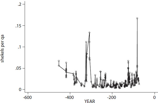
FIGURE 3.1. The price of barley, 464 to 72 BCE
Source: Slotsky (1997)
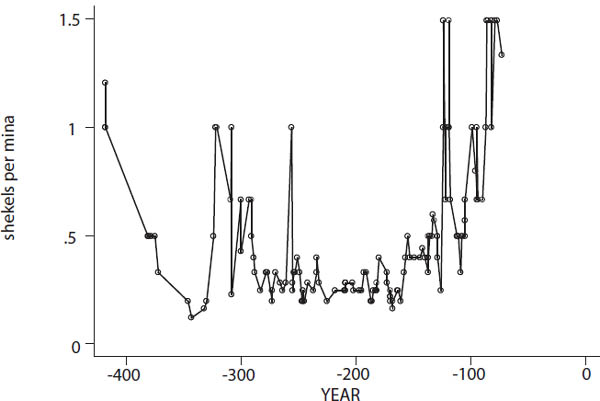
I study the data from 464 to 72 BCE, omitting one stray set of market values for 568 BCE. The data contain many missing values because of the many lost tablets and the large number that are damaged or broken. The commodity summary was inscribed close to the end of a monthly unit. The last month on a tablet was at the bottom of the tablet and in a particularly vulnerable position; there are many disconnected and broken passages, not to mention lost quotations. Tablet damage and loss was random from the point of view of prices. There are over three thousand observations—almost as many observations for each of the six commodities as Hopkins (1978) found for all slave freedom prices. The prices of barley and wool are shown in figures 3.1 and 3.2. Barley prices are measured in qa (close to a modern quart) per shekel (a standard weight of silver). Wool prices are measure in mina (close to a modern pound) per shekel.
Slotsky (1997) had no doubt that the market quotations were real market prices. The texts contained principally observed rather than predicted phenomena. The quotations appeared too irregular to have been computed according to some abstract principle. The pace of reporting commodity prices quickened and became erratic when they were volatile, and there were reports of interrupted or suspended commodity sales at these times. Slotsky analyzed these putative prices in the manner of an ancient historian and philologist, although she did use some statistics. I have used the tools of economics to ask if these magnitudes behave like real prices. If so, what can we learn from them about the economy of the classical world?
FIGURE 3.2. The price of wool, 464 to 72 BCE
Source: Slotsky (1997)
Grainger (1999) and Van der Spek (2000) interpreted these prices as market prices. Grainger described long-run trends, and Van der Spek argued that prices rose in wartime. Grainger based his argument on bar graphs, while Van der Spek cited isolated prices, restricting his observations to wartimes and to the price of barley. Neither author subjected the data to any kind of formal tests.
In order to create a frame of reference, I compare the Babylonian prices with the price of wheat in England during the medieval and early modern periods. The price of wheat is a good standard of comparison for several reasons. The wheat prices are well attested and continuous for centuries, comparable to the Babylonian prices. They are the prices of an agricultural commodity from a primarily agricultural economy, as are the Babylonian prices. And they clearly were set in relatively free market conditions.
The first question is whether the Babylonian prices are market prices. To answer that question I need to consider what else they might be. The alternative is some sort of administered prices that indicate nonmarket activity such as tax collections or royal exactions of some other sort. If these prices indicated such an administrative activity, they would have been generated by some rule and would have followed a uniform pattern like the celestial movements also recorded on the tablets. Market prices, by contrast, move freely in response to changing conditions and would have exhibited a far more random pattern.
I therefore can test for market prices by looking for random movements in the data. I distinguish five types of movements to be examined.
1. Annual variation. I measure the year-to-year variation by examining yearly prices. Only the year in which prices were reported is relevant here, not the month. As can be seen from figures 3.1 and 3.2, the price series exhibit substantial annual variation. Prices, as we know from the modern world, also exhibit autocorrelation. In fact, they typically can be described as a random walk.
2. Long-run variation. I examine trends over time to see if prices exhibited persistent trends over the four centuries I observe. Administered prices could remain constant over time, but market prices are more likely to exhibit inflation or deflation over this long period. Grainger (1999) inferred long-run trends from bar graphs but could not test for significance in light of the short-run variation.
3. Short-run variation. Market prices react to unexpected events. Alexander returned to Babylon in 324 BCE and then died suddenly in 323, giving rise to lasting dynastic conflicts. These were events of great magnitude. If these observations are market prices, they may well have shown some effects. Changes in the supply of silver and any scarcity of goods resulting from Alexander’s death both could have caused prices to rise. Van der Spek (2000) interpreted a price rise at this time as the effect of war rather than of other events.
4. Relative variation. The scribes recorded prices for six commodities. If the prices were administered, they should have preserved their relative magnitudes. It is a hallmark of administered prices even in modern times that they do not vary against each other (Berliner 1976). Market prices, by contrast, often diverge as there are changes in individual markets. Five of the prices I have are for crops, while wool is an animal product. If these are market prices, the price of wool could have moved differently from the price of crops.
5. Seasonal variation. Agricultural prices tend to have patterns that reflect growing conditions, both seasonal variation within years and yearly variations from weather changes. Crops were harvested at different times of the year in ancient Babylon, and there may not be uniform seasonal patterns. In addition, there may have been good and bad years for agriculture as a whole.
I use the annual variation of prices to test whether these prices were generated in relatively free markets. The prime characteristic of such prices is that they are not predictable in the short run. In other words the best prediction today of what a price will be tomorrow is the price today. The stock market today seems to be the best example of prices like these. The evening news reports whether prices went up or down. The news is based on the assumption that prices are autocorrelated, that is, that today’s price is correlated with yesterday’s price. It also is telling us what we could not have known yesterday, how today’s price differed from yesterday’s price. The change from yesterday was random from yesterday’s point of view.
We speak of stochastic processes like this as random walks. The variable “walks” like a person, starting off from the results of the previous step and moving randomly to the next step. We therefore can express this movement in an equation that says that today’s observation is equal to yesterday’s observation plus a random movement. In the case at hand, today’s price is equal to yesterday’s price plus a random amount. It is possible to talk of a random walk with drift, as you can observe for prices in the midst of inflation or deflation. In that case, the randomness comes from the expected deviation around the trend, not simply from the previous price level.
In order to make the results intelligible and accurate, I make two changes in the price data as they are found on the tablets. They reported the quantity of barley, for example, per unit of currency. We are used to thinking about the units of currency needed to buy a standard unit of barley. I therefore use the inverse of the prices listed by the priests from the Temple of Marduk. I also use the logarithm of prices in order to reduce the effects of outliers in the data and to make the random movements independent of direction.
In order to deal with holes in the data, I have to expand the standard equation for a random walk. Despite the abundance of Babylonian prices, there are not prices for every year. There are more than three thousand observations, but they are for six commodities. That means about five hundred observations for each commodity, spread over roughly four hundred years, and there are not enough surviving tablets to provide observations for each year. To account for any possible trend in the prices, the trend needs to be multiplied by the number of years since the last observation. Since I am using the logarithm of the prices, the coefficient on the previous price needs to be raised to the relevant power.
I examine the first kind of variation through regressions of the following form:
Log Pricei(t) = α + βiLag (t) Log Pricei(t – 1) + ε(t)
For modern prices with annual observations, Lag (t) = 1 for all years, and it normally is not expressed. As noted above, I calculated the price as the inverse of the volume or weight measure of each commodity described earlier.
TABLE 3.1.
Regressions of log prices on last year’s prices
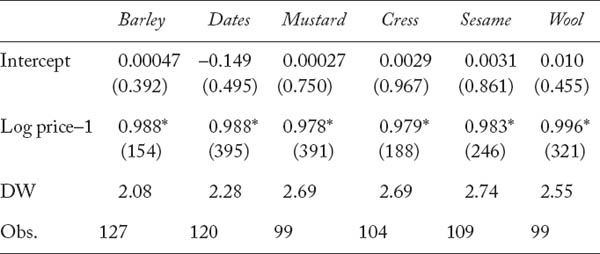
Absolute values of t-statistics are below the coefficients.* = significantly different from zero at 1% probability.
The results of estimating this regression for each of the six commodities are shown in table 3.1. In each case, the constant is close to zero, and the coefficient on last year’s price is very close to one. Taking into account the randomness of the sample of prices that have survived, as in chapter 2, the small standard errors of the coefficients show that the constant is not significantly different from zero nor the coefficient on the lagged price different from one. In plain English, the probability that the constant is different from zero or that the coefficients are different from one is less than 1 percent. These prices describe a random walk very much like that of modern prices.
I compare the autocorrelation in agricultural prices from Hellenistic Babylon with that in medieval and early modern English wheat prices to see if the degree of autocorrelation is the same. The analogous regression for wheat prices from 1260 to 1914 is:
Log Pricew(t) = –0.042 + 0.942 Log Pricew(t–1) + ε(t)
(0.28) (67.3)
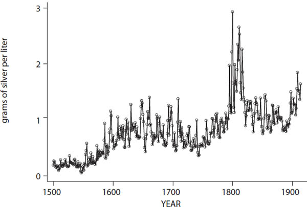
Lag (t) has been suppressed since there are no missing years in the data and “t” in this expression always takes the value of 1 in this regression. The price of wheat for early modern Britain shows exactly the same kind of autocorrelation as the ancient Babylonian prices. The price of wheat after 1500 is shown in figure 3.3, using only part of the modern price series to approximate the time interval of the ancient one. The graph looks very similar to figures 3.1 and 3.2.
The existence of this stochastic process is a clear marker for market prices. The ancient prices behave like medieval and early modern prices, which in turn share the time-series properties of prices today. Administered prices could not possibly have these properties. They would stay at or near some fixed level, or a level that changed deterministically over time; they would not behave as a random walk. In the regression, the constant should have been at the administrative level and clearly not zero, while the coefficient on the previous price would be zero. The data in figures 3.1–3.3 and table 3.1 therefore document clearly the market nature of agricultural prices in Babylon before and during the Hellenistic period.
FIGURE 3.3. The price of wheat in England, 1500 to 1914
Source: Allen (2001)
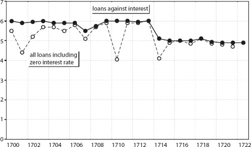
To make the comparison more vivid, I show an administered price from eighteenth-century London in figure 3.4. The usury rate was binding at this time, and this figure shows the interest rate charged by a London bank to its customers. The usury rate was lowered from 6 to 5 percent in 1714, and the rate charged by the bank fell by the same amount. In a regression for the rates charged by the bank, the constant showed up as 5 or 6 percent depending on the date, and the coefficient on an unregulated interest rate—the return on government bonds—was effectively zero. To emphasize that these were actual rates, I added in a dotted line the average rate the bank charged, including loans that were made without any interest charge at all (Temin and Voth 2008).
This conclusion can be strengthened by analysis of the path of these market prices over time. As can be seen in table 3.1, the number of observations for each commodity fell from the observed five hundred or so to one hundred or slightly more in the annual regressions. This was the result of collapsing the data into annual observations and allowing for lags, and the remaining observations are quite sufficient to demonstrate the time-series properties of the ancient data. I used all the observations for the descriptive regressions described in the appendix to this chapter. These regressions summarize the movements of the prices in variations 2 through 5 and illuminate patterns shown in figures 3.1 and 3.2. See the appendix for regression specifications and partial results.
FIGURE 3.4. Two “average” interest rates, Hoare’s, 1702–25
Source: Temin and Voth (2008)
The results of estimating further regressions for each of the six commodities indicate that a cubic equation captures well the curvature of the price series. The presence of all positive coefficients appears to indicate steadily rising prices, but dealing with years before the Common Era is tricky. The years before the Common Era are negative, increasing from –463 to –71. As the years progress, getting closer to zero, the effect of a positive sign on a negative year diminishes, and prices turn upward. The prices of three commodities—cress, mustard, and dates—rose initially in the fifth century BCE, then fell until shortly after 200 BCE when they began to rise again. The prices of wool, sesame, and barley fell from the earliest years observed until reaching a minimum between 250 and 200 BCE, after which they too rose. Prices moved in various ways in early years, but they all rose with increasing speed after 150 BCE.
Grainger (1999) attributed this inflation to the breakdown of the Seleucid state. A lack of public order could impede trade and make goods scarce. But this argument about the demand for goods ignores the supply of money; an abundance of silver also could cause commodity prices in silver units to rise. We can clarify the problem by referring back to the supply and demand analysis in chapter 1. It is easiest to examine the supply and demand of silver, the units in which Babylonian prices were given. The price of silver is the inverse of the price of the commodities as noted earlier. When prices go up in inflation, the “price” of money, that is, silver, goes down.
Was this due to a shift in the supply or demand for silver? Grainger argued that the demand for silver went down because there were not enough goods to buy. People wanted goods and were willing to pay lots of silver for them. But what was happening to the supply of silver? We do not know much about the supplies of silver in this period, because most of our information comes from examining coins. Commerce in Babylonia was not based on coins, but rather on standard weights of silver. When Alexander introduced coins, they were weighed rather than counted (Powell 1996; Vargyas 2000). It is very hard to know how many coins were circulating, and even harder to estimate the volume of silver in use.
Alexander established a mint in Babylonia around 330 BCE when he first arrived. He then went to Persia and beyond, returning with treasure in 324, presumably including silver. But we do not know how he financed his expedition, and there is no evidence that the Persian treasure was made into coins (Mørkholm 1991, pp. 48–49). Conventional wisdom is that Rome was taking silver from the East in taxes and tribute. The Roman Republic was expanding its use of silver coinage in these years, and “silver drained out of Spain and the Greek world” to Italy and Rome after 200 BCE (Harl 1996, p. 39). It is unlikely as a result that there was an increasing supply of silver in Babylon. In addition, when Augustus reformed the Roman currency a century after the Babylonian price series ends, his coins embodied a gold-silver ratio of 12:1, valuing silver higher relative to gold than it would be valued later (Greene 1986, 49). This evidence does not suggest an abundance of silver in Rome at the end of our period, making a prior expansion of silver supplies in Babylon even more unlikely. Grainger’s suggestion therefore appears to be a reasonable one.
A more rapid and more short-lived inflation took place in the years after Alexander’s death. Prices rose dramatically and took about a generation to return to their normal trend. This price rise, clearly visible in figures 3.1 and 3.2, reveals the market nature of these prices, since episodic price rises are hallmarks of free markets. As with the later, more gradual price rise, the cause of this rise can only be inferred indirectly. It appears to be the effect of Alexander’s unexpected death and the dynastic conflicts that followed.
If so, what was the mechanism? As in the more gradual later inflation, prices could rise either because agricultural goods were scarce in Babylon or because the stock of silver suddenly rose. Alexander brought back with him extensive plunder in 324 BCE. He did not coin this treasure, as noted above, but one modern author argued that he “released [his treasure] into circulation,” dramatically increasing the supply of money (Patterson 1972). It is likely, however, that Alexander did not by himself give rise to this short, sharp inflation. Instead, competing claimants to Alexander’s throne probably paid their soldiers from Alexander’s treasure during the dynastic struggles that followed his death. Stolper (1994) described the political history of these years, showing that the dynastic conflicts continued for a long time. It is the continuation of these struggles that explains why prices stayed high for a generation after Alexander’s sudden death. Of course, the inference that an increased supply of money caused prices to rise assumes that the prices in question were market prices determined in reasonably well-functioning markets.
The supply and demand model of chapter 1 has enabled us to distinguish between the two bouts of inflation in the Babylonian prices data. The swift inflation and deflation after Alexander’s death was caused by changes in the supply of money, while the more gradual inflation starting in the second century BCE was due to changes in the demand for money. In other words, these two inflations were very different phenomenon with very different causes. One role of economics is to clarify the nature of the events that we observe. I discuss more statistical results in the following paragraphs; the regressions themselves are explained in the appendix to this chapter.
The analysis done here shows that agricultural prices in Babylon moved randomly from year to year, fell and rose again over the long run, and experienced severe market disruption after the death of Alexander the Great. These conclusions imply more general conclusions about ancient Babylon. There clearly were markets for agricultural goods that were operating continuously and giving rise to market prices. This suggests that there was a market economy in ancient Babylon. To reach a stronger conclusion about the economy as a whole, we would need evidence on the spread and influence of other markets as well as the ones analyzed here. I argue in this book that there was a market economy in the early Roman Empire by examining the nature of markets for commodities, land, capital, and labor. We lack this knowledge of the extent of market behavior in pre-Hellenistic and Hellenistic Babylon. We therefore can only be sure that there was a functioning free market in agricultural commodities.
The movements of these prices over time suggest conclusions about the politics of ancient Babylon as well. The severe disruption of prices after the death of Alexander confirms the views of those historians who have seen his death as the end of an era. The regressions tell us that it took almost a generation to restore stability to the agricultural markets in Babylon. They inform us that it was not a simple thing to restore order after a sudden shock like Alexander’s death. The succession may have been decided quickly, but life did not return to normal for many years.
After order was restored with the establishment of the Seleucid dynasty, prices appear to have stabilized. But in the last two centuries before the Common Era, prices began to rise. As discussed earlier, this inflation may indicate a gradual breakdown of the government’s ability to maintain stability as the Seleucid Empire gradually disintegrated. This price evidence, like that for the later Roman Empire, suggests that political and economic stability were becoming harder to achieve as time went on. A more complete analysis of the Roman inflation is presented in chapter 4.
The results of estimating equations for each of the six commodities revealed that the prices for different commodities differed from each other. There were trends in relative prices as well as trends in the price level as a whole. This again reveals agricultural markets in action. Only administered prices maintain their relative prices over long stretches of time. Wool in particular followed a unique time path, as suggested by the contrast between figures 3.1 and 3.2.
In the years around 100 BCE, the price of wool rose when the price of agricultural crops did not. There were high wool prices in several years, spaced over a few decades, although there also were some lower wool prices interspersed. These high observations affect regression trends, although they also may have represented a more short-run movement. It appears that there was some kind of wool shortage or disruption of the wool market at the end of the observed period. The statistical work reported here cannot identify the cause of this disruption; it can only identify the existence of something unusual in the wool market.
Seasonal dummies reveal a complex pattern, which I describe without reproducing the full regression results. Dates were delivered in the fall, and date prices were lower in the following half year than in the half year before the harvest. Barley was delivered in the spring, and it was more expensive in the preceding few months. But although mustard was delivered in the fall like dates, it was more expensive at the same time. The other three prices did not have seasonal patterns that can be recovered from the data with confidence. Approximately two hundred observations on the height of the Euphrates have survived, but only about one hundred of them overlapped price data on each commodity. Regressions of log prices on years and the height of the Euphrates did not reveal a significant effect of the river height on any of the six prices. The seasonal evidence therefore is ambiguous. There is some evidence that fits a model of an agricultural economy, but also seasonal evidence that does not.
Taking all these observations together, I reach two conclusions. First, careful analysis of these prices using time-series techniques confirms the conclusion in Slotsky (1997) that these prices were market prices. They moved with a great deal of randomness, and they varied over time. These agricultural prices moved like the random walk of modern prices, and they varied together in response to weather that affected all crops. These changes are understood clearly within a market framework; they are impossible to understand within an administrative one. I conclude therefore that the scribes recorded prices set in functioning markets.
Second, the pattern of prices informs us of economic conditions in Babylon before the Common Era. Prices fluctuated a lot. The return and subsequent death of Alexander led to a major shock to the supply of money and therefore to prices, sustained for a generation or more. Prices rose sharply and stayed high; normal conditions did not return for more than twenty years. This price disruption indicates how hard it was for political and economic stability to return, how hard it was to reestablish peaceful conditions where foodstuffs were available cheaply. People living in Babylon during this transition must have had a very difficult time. It appears that food was twice as expensive as usual in the city of Babylon; it is unlikely that most urban dwellers had assets that enabled them to offset the scarcity of food. Farmers by contrast may not have been affected if the prices they received for their produce rose as much as the prices of products they bought.
Prices rose in the last two centuries before the Common Era, gradually at first and then with increasing speed. This inflation suggests a gradual weakening of the political structure in Babylon in the final centuries before the Common Era since there does not appear to have been a shock to the money supply in these years. A gradual inflation does not indicate as much hardship for ordinary people as the sudden price rise of years before 300 BCE. Wool became expensive at the end of the period relative to other products, with prices that rose beyond the rise of other prices. This may have been a hardship for many people and possibly a boon for a few. Only future research can discover the cause of this price inflation and its possible effects on the lives of ordinary people.