There is growing evidence that ordinary Romans lived well in the early Roman Empire. The existence of many cities, and particularly the large size of Rome itself, provides indirect evidence of productivity advance. More detailed evidence is emerging of improving agricultural technology, building techniques, manufacturing plants, and land use. The widespread use of African Red Slipware pottery provides evidence that even ordinary people had access to the fruits of all this technology. And the literary evidence supports the idea of prosperity by providing insights into civilized urban lives in Roman cities. As explained in chapter 9, these are all proxies for economic growth. They are not measures, but they are suggestive. How could per capita income grow in a Malthusian economy? This chapter resolves the apparent paradox of economic growth in a Malthusian world.
Even if this evidence of an improvement in general living standards is not yet convincing to everyone, there by now is enough evidence to raise the possibility that such a movement might have taken place. In the spirit of Morley’s (2001) essay on the implication of a large Roman population, this chapter offers a way to understand rising per capita incomes in Rome as the accumulating evidence becomes persuasive.
It seems paradoxical that we have evidence of a rise in per capita income when we face so much uncertainty about the size of the population whose income is growing. This is only partly a matter of evidence; it also is a result of our theories. We assume that the scattered evidence of living standards can be generalized to larger groups because we implicitly or explicitly assume that people lived at roughly the same level. This does not mean that we ignore class divisions in Rome, but that we compare the lives of ordinary Romans with their predecessors. We assume this similarity of income for working families because we assume there was a labor market that brought wages into some kind of rough correspondence. I argued in chapter 6 both that we need to make such an assumption to make sense of a lot of the modern literature on ancient Rome and that this assumption is an accurate one in the early Roman Empire.
FIGURE 10.1. World economic history in one picture
Source: Clark (2007a, 2)
The problem with theories is that there are lots of them. We use the theory of competition between workers to support the idea that living conditions improved in the later republic and early empire, but the Malthusian theory of population change argues that our observations must be false. In that theory, changes in productivity lead to changes in the size of the population (which we cannot observe) and leave the level of per capita income (which we do observe however imperfectly) the same. The implications of this theory can be seen in figure 10.1, taken from a new economic history of the world. The level of per capita income is assumed to be roughly constant before the Industrial Revolution. Saller published a more abstract version of this graph making the assumption of constant per capita income before the Industrial Revolution more apparent. He did not allow for the fluctuations around this level indicated in figure 10.1 (Clark 2007a, chapter 1; Saller 2005). This figure has just reemerged in a new book about a “unified theory” of economic growth (Galor 2011).
The view in figure 10.1 is too reductionist for the analysis of the Roman economy. From the twenty-first century, events before 1800 appear to merge together, and it is useful to summarize them in a simple way. This tendency leads historians to interpret the Malthusian model very strictly, but there are important delays in the Malthusian system. These dynamics are integral to the Malthusian model, and historical evidence from other periods indicate that the delays can be exceedingly long—on the order of centuries rather than decades. These dynamics provide a way to acknowledge growing per capita income in the basically Malthusian world of the early Roman Empire. It also provides a way to ask if the Romans could have escaped—in some alternate history—the Malthusian constraints.
I start this argument by reviewing the evidence that per capita income was high and that it fell as the Roman Empire disintegrated. I then explain how the Malthusian model works with attention to the dynamics of how shocks affect both population size and its income over time. The model reveals how an economy could avoid the Malthusian constraints within this Malthusian model for an extended period. Breaking out—industrializing—is a different matter, and I close with some speculations about the nature of the Industrial Revolution and its relevance for Roman history.
Finley (1973) argued that the ancient economy was dominated by stagnant technology. This view became the one that historians of later periods saw when they looked back at the ancient world. In a book about the history of technology in the Western world, Mokyr (1990) spent a chapter trying to explain Roman technological stagnation.
The tide has changed in the last decade. Roman archeologists have found abundant evidence of new technologies in the Roman world, and their views are now appearing in print. Greene (2000) started the debate with a paper challenging Finley on several grounds. He argued that Finley had been misled by the literary sources; only archeology could show how technology had improved. Wilson (2008) expanded the case for a progressive Roman technology in several papers, and I follow his lead here. I discuss in turn the growth of regional specialization, the expansion of land for agricultural purposes, manufacturing, and construction.
Everyone knows about the Pax Romana. Pompey finished clearing the Mediterranean of pirates in 67 BCE and made safer transport possible. The risks before then are illustrated by the kidnapping of Caesar and its subsequent horrifying effect (Casson 1991, 181–83). The usual interest in this story is Caesar’s insolence toward his captors and his subsequent revenge. I emphasize here the risk of capture that is the premise of the story. As North (1968) argued in a paper cited by the Nobel Committee in awarding him the Nobel Prize in economics, reducing the cost of defending against pirates lowers the cost of shipping.
A lower cost of shipping allowed production to be located around the Mediterranean where conditions were most suitable. Instead of growing wheat in Italy, inhabitants of Rome ate porridge and bread made from wheat grown in Sicily, Egypt, Africa, Spain, and other places. Production was scattered because it was more efficient to grow wheat in these places than in Italy. Romans did not calculate what we call efficiency; instead they purchased wheat where it was cheapest. It was cheapest in places where grain agriculture was the best use of land and labor resources (Erdkamp 2005, chapters 2, 5; Rathbone 2009, 322).
The gain to both the exporting and importing regions was shown by Ricardo in his theory of comparative advantage and explained in chapter 1. Trade that allows regions to specialize in what they produce best increases the income of both sending and receiving regions. Trade functions like an extension of resources in any one region; it loosens the constraint of limited land in an agricultural economy. One effect of Roman regional specialization was the shift in Italian farms from wheat to other crops that did not travel as well (Morley 1996; Geraghty 2007).
Roman roads performed a similar service to the economy. They were less important than a peaceful sea because overland transportation was much more expensive than water-borne transport. In addition, the roads were built for military reasons; any commercial use was incidental. The roads nevertheless made it easier for goods to get around. They promoted local specialization similar to the broad patterns just described. They also allowed goods brought from far away to reach consumers living away from seaports. Shipping and roads therefore both promoted a better life for Roman citizens.
They allowed the Romans to create the urban society that was unique in the ancient world. The agricultural system—including agriculture, trade, and coordinating institutions—was efficient enough to release substantial numbers of people from the tasks of growing food. These people could gather in cities, and they could produce other goods and services. These added products improved the quality of Roman life, and they added to per capita income.
In addition to gains from regional specialization, there was technical change in each place. Mokyr (1990, 23) opened his book on technology with a chapter that criticized Finley for being too pessimistic, but he still argued that “new ideas were not altogether absent, but their diffusion and application were sporadic and slow.” Recent archaeological discoveries dispute that conclusion.
Terracing was common, extending the range of land on which crops, particularly grapes and olives, could be grown. Wine and oil presses also used the screw, enabling grapes and olives grown on new land to be processed more efficiently. The Archimedean screw was used widely in cereal agriculture to drain land, extending the range of land that could be used for this crop as well. Our evidence is spotty, but recent archaeological discoveries from many different areas suggest strongly that these innovations had diffused over large ranges of the Roman Empire (Wilson forthcoming).
Everyone knows about the Roman use of arches and concrete to construct buildings, roads, and ports. Transportation helps to achieve gains from trade as well as enhancing productivity in other ways. Aqueducts are well known, but the sophistication needed to construct them seldom is noticed. In addition to the construction of the aqueducts, the level had to be adjusted for water to flow over often large distances. Only a little thought is needed to realize that the widespread evidence of aqueducts provides evidence of the diffusion of engineering knowledge around the Roman Empire.
Water wheels also were more prevalent in Roman times than previously thought: “Today, we may state with confidence that the breakthrough of the water-powered mill did not take place . . . in the early middle ages, but rather . . . in the first century A.D., or perhaps even slightly earlier” (Wikander 2008, 149). And mass-produced Roman products were prevalent: “Pottery, glassware, bricks, coins, plate, and humble metal objects such as nails were produced in enormous quantities to standard shapes and sizes, and widely traded around the Roman Mediterranean and northern Europe” (Wilson 2008, 393).
Yet the evidence of technical change is not quite the information we need. Greater production expanded the resources available to feed people, but it could have resulted in more people rather than higher per capita incomes. As noted in chapter 9, population often is used as an indication of early growth over the long run. The Roman Empire lasted for several centuries, but the time frame of the Malthusian model is even longer. The purpose of a model is to show how individual incomes could have changed in the short run.
We need evidence on the consumption of ordinary people to show that they were better off as opposed to more numerous. Any society can support an elite that lives well; richer societies can have large elites. These elites typically are too small to affect the growth of the population as a whole, although the Roman elite was quite large. We need evidence that extends beyond the literary evidence of sumptuous Roman dinner parties and feasts.
Diet is an important part of the consumption of ordinary people and therefore a good indicator of the standard of living before the modern rise of per capita incomes. The consumption of wheat was enhanced by making it into bread rather than porridge. The Roman conquest and the resulting reduction in transportation costs led to an increasing variety of diet, including a wide range of new fruits and vegetables. More important, there is evidence of greater meat consumption in both Roman Italy and the provinces. Meat, of course, is a superior good, and its consumption rises with per capita income. There were more animal bones in the early Roman Empire than in surrounding centuries, and the number of animal bones peaks again around 500 in Roman Italy. Animals were larger in this period than before or after, adding to other suggestive evidence of improved diets and higher incomes (Jongman 2007b).
Ordinary people also had consumer durables that were better than those before or after. The most prevalent was African Red Slipware, ordinary pottery that is found everywhere in Roman settlements. The pottery was wheel-thrown and highly fired, supplying a “modern” platform on which to eat. In addition to plates, ordinary people had iron knives with which to cut their food. Good Roman pottery contrasts sharply with the friable pottery found in post-Roman Britain that was neither wheel-thrown nor highly fired. The comparison shows the decline in the living standards of ordinary people after the Romans left Britain. There must have been a previous rise in per capita income for it to fall sharply thereafter (Ward-Perkins 2005).
The omnipresent oil lamp was another consumer durable of Roman times. It extended the day and enhanced the quality of life in interior spaces for many people. The assemblages of oil lamps in many museums show their spread throughout the empire and the standardization that reveals their industrial origin (Harris 1980). Like agricultural goods, industrial goods were made in centralized locations and shipped all over the Roman world.
Evidence of widespread improvements in consumption is increasing, and Roman citizens must have had increasing incomes to buy the enhanced food and consumer durables. Jongman (2007b) cited a variety of estimates showing that real wages increased in the late republic and early empire. He surveyed the occasional evidence of documented wages, subsistence annuities, and slave prices—as an index of wages of free workers with whom Roman slaves competed. The data for any one of these measures are spotty, but the pattern of all of them is the same. This common pattern suggests that the occasional observations are capturing underlying trends whose existence is attested to by the variety of evidence that fits the pattern. Real wages rose after the Antonine Plague. Labor income was the major part of total income in the agrarian society of ancient Rome, and an increase in real wages is a good index of an increase in total income.
Allen (2009a) used data from the Diocletian Price Edict of 301 to compare real wages in Rome with those in early-modern European and Asian cities. He found that the real wage calculated from the Price Edict was close to the real wage in Florence in the eighteenth century. This is impressive for an ancient society, but it also is less than real wages at the same time in London and Amsterdam and less than Florentine real wages in the century after the Black Death. Scheidel (2010) replicated Allen’s estimations for Roman Egypt.
The evidence for enhanced consumption is still very sketchy, and we hope that archaeologists will broaden the evidentiary base over time. Enough evidence has been found already to indicate that ordinary Romans lived better than ordinary people before or for many centuries after. The problem is how to square these observations with the iron law of subsistence living that is part of the Malthusian model of population change.
In particular, this evidence suggests that living standards for ordinary Romans improved in the late republic, reaching a high standard for the early empire. Given the long history of the republic, this growth did not have to be rapid to result in a substantial increase in living standards. It did, however, need to be sustained over the course of a century or more. How could these innovations result in rising living standards rather than simply more people? We need to examine the Malthusian model of population dynamics to see.
Malthus argued that the size of the population was limited by the resources available to feed it. By resources, most people now mean land, understanding that the use of land and other resources may be relevant as well. This Malthusian relation is known to economists today as the declining marginal product of labor when the number of workers on a given plot of land increases. This, of course, was Ricardo’s way of making the same point at approximately the same time as Malthus, and it is Ricardo’s formulation that has become central to modern economics; as the number of workers rises, wages fall and rents rise (Malthus 2004).
Wages in this summary mean “real wages,” that is, the purchasing power of wages as described by Allen (2009a) and Scheidel (2010). The diet of most workers near a Malthusian equilibrium consisted largely of grain in one form or another. We therefore approximate the real wage by looking at the ratio of the money wage to an index of the price of goods workers bought, weighting grain heavily in this index. If we divide money wages by the price of grain alone, we get a measure of the marginal product of labor, since farmers typically hire workers up to the point where the last (marginal) worker produces just enough grain to pay for the wages he earns (Clarke 2007b).
Ricardo’s formulation shows the need for an additional relation for Malthus to find an equilibrium point on this line. Malthus did this by specifying a relation between worker’s wages—taken to be their income—and their birth and death rates. Births rise with income, both as nutrition rises and as younger marriages become feasible. Death rates fall with income as infant mortality declines and plagues, wars, and pestilence become less frequent. Modern research has confirmed the first of these relations, while generally failing to find convincing evidence of the latter (Lee 1980). For most purposes, only one relation is needed, provided the other one does not operate in the reverse direction. The full Malthusian model then was taken to restrict the range of early history. Wrigley’s (1988, 29) description of the world before the Industrial Revolution is clear: “An organic economy, however advanced, was subject to negative feedback in the sense that the very process of growth set in train changes that made further growth additionally difficult because of the operation of declining marginal returns in production from the land.” Clark’s (2007a, 27) recent description is equally clear: “Anything that reduced the death rate schedule—advances in medical technology, better personal hygiene, improved public sanitation, public provision for harvest failures, peace and order—reduced material living standards.”
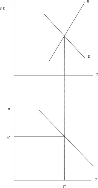
The preceding discussion is summarized in figure 10.2. The horizontal axis on both graphs is the same: per capita income. The top graph shows the determination of population size. Population grows if births exceed deaths; it falls if births fall short of deaths. The equilibrium is where the birth and death rates are equal, at y*. The bottom graph shows that the resource constraint permits only a limited population size, n*, at this income. Note that the model works well even if there is no relation between income and the death rate. If the curve marked D in the top graph is horizontal—that is, if it shows the death rate unaffected by changing income—y* is still the equilibrium, and the analysis proceeds as before (Lee 1980; Clark 2007a, chapter 2).
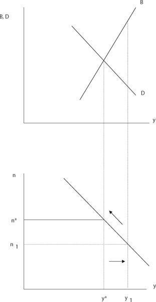
Consider the effect of a plague, like the Antonine or Justinian plagues, in this model. Let us assume that the population fell by approximately one-third, without aiming for spurious precision. The effects are shown in figure 10.3. Population fell from n* to n1. As population fell, income rose above the previous equilibrium income, y*, because the marginal product of labor rises as population falls. At this higher income, n1 in figure 10.3, birth rates exceeded death rates, as shown in the upper graph. Population grew as a result. It continued to grow until income was reduced to its previous level, y*, where births and deaths were once again equal. As can be seen in the lower graph, per capita income was unchanged at the new equilibrium, and the population returned to its former size.
How long did this process take? From the long-run point of view of figure 10.1, this may not be important, but if it took a long time to return to y*, then per capita incomes may have been above that equilibrium level for some time. According to Solow (2007, 39), Nobel laureate in economics, “The Malthusian process works itself out slowly. The chain of causation . . . could take years or decades to complete itself.” Is this accurate, or is even this casual estimate of the delays too short?
We do not have much evidence from the Roman plagues, but we know more about the aftermath of the Black Death of 1349 in England. Immediately after the plague, money wages of farm workers shot up. As I argued for the Antonine Plague in chapter 4, the immediate effect of a plague is inflation. Wages and wheat prices both rose. Yet for the Malthusian model we need to know the path of real wages, that is, the extent to which the rise in money wages exceeded the rise in the price of grain and other consumables.
Clark (2007b) provided detailed information about the progress of English real wages after the Black Death. He showed that real wages did not rise nearly as fast as money wages in the immediate aftermath of the plague. Instead they rose gradually and peaked a century after the plague, in the middle of the fifteenth century. Malanima (2007; 2009, 264) replicated this finding for Italian agricultural real wages, showing that they also peaked around 1450. Allen’s estimated English real wages, reported by Malanima for comparison, peaked even later than shown in Clark’s data, perhaps as late as the end of the fifteenth century. It is clear that the population did not recover to preplague levels for over a century. It took a very long time for the Malthusian system to return to its equilibrium. Clark was interested in the return to the equilibrium—as shown by figure 10.1—while I am interested here in the deviations from it.
FIGURE 10.2. The basic Malthusian model
FIGURE 10.3. Effect of a plague
It cannot be surprising that the return to the Malthusian equilibrium took a long time. Initially, the disruption of the plague delayed economic adjustment to the new factor proportions. As discussed in chapter 4, plagues lead also to inflation, explaining why nominal wages rose immediately after the Black Death. Only gradually did farmers take advantage of the increased land per worker and increase their incomes. Higher incomes after the Black Death may have resulted in earlier marriages, which in turn led to more children. But it took a generation or more for the effects of this change to become apparent in the agricultural labor market. If women changed their behavior slowly, it might take several generations to lead to population expansion. And when we start talking about generations, it requires only a few generations to make a century of delay. While we do not know much about family dynamics in the late fourteenth century, we do know that real wages did not start to fall until a century after the Black Death.
This is consistent with the limited evidence from the Antonine Plague. Scheidel (2002) collected fragmentary wage and price data from Roman Egypt in the second and third centuries. The ancient sources are not frequent enough to provide the detailed timing evidence found in the medieval data, but they suggest a long period after the plague when wages were high. If we regard the observations as random draws from records of wages and prices in the two centuries, we are implicitly assuming that the effects of the population decline in the Antonine Plague lasted as long as the decline after the Black Death. According to Scheidel, however, the rise in the real wage, that is, the ratio of wages to commodity prices, was smaller in the ancient world. Real wages were less than half again as large in the third century as in the second century, while real wages peaked at twice the preplague level in the fifteenth century. More ancient evidence would help us calibrate both the timing and magnitude of the ancient shock.
As a matter of logic, real wages had to rise as part of the demographic process. The question for ancient history is not whether individual incomes grew, but rather how much and for how long. Scheidel’s (2010) recent estimates of real wages in Roman Egypt fail to show any rise following the Antonine Plague. The difference appears to come from the choice of deflator, whether wheat alone is used (to maximize the number of historical observations) or a basket of consumption goods (to maximize the fit with the modern methodology described in chapter 9). The best view at the current time is that there was a significant demographic event called the Antonine Plague, although its economic effects still are only dimly seen and apparently more modest than those of the Black Death.
Consider now a different shock to the Malthusian system. Instead of assuming that the size of the population changed, assume that the Malthusian resource constraint shifted outward. This change could come from regional specialization permitted by the Pax Romana. It could come from technological change that allowed land to be used more efficiently as described by Wilson. In any case, it shifts the line in the bottom graph of figure 10.2 to the right. For any given population size, the available land now allows the marginal product of labor and income of farm workers to be higher than before.
As shown in figure 10.4, this sets up a population expansion. In the short run, the effects of this positive shock are the same as the results of a plague shown in figure 10.3, but for different reasons. The population changed dramatically during a plague, but it changes more slowly under normal conditions. Per capita income can change more rapidly, and it increases in the short run, leaving population unaffected. But in the longer run the equilibrium has changed. The excess of births over deaths causes population to rise. Equilibrium is reached when income returns to its previous level in the upper graph, y*. Looking at the lower graph, we see that the population is larger at the new equilibrium than before, at n2 instead of n*. The effect of technical change has been to increase the size of the population, not per capita income, in the Malthusian equilibrium.
Note the differences between figures 10.3 and 10.4. In both of them, income rises, setting off an increase in population. This is a rightward shift in both graphs. Although population grows in both graphs, the relation of this growth to the prior level of the population is different. In figure 10.3, the population is always lower than n*, and the growth is only to regain the losses from the plague. In figure 10.4, by contrast, population is always larger than n*, as technology allows for a larger population. If the shift in the resource constraint is a one-time movement, then the population settles down to a new equilibrium level, n2, larger than n*.
As before, the economy will not move instantly to this new equilibrium. It will take a long time, perhaps more than a century. During that time, per capita income will be high and population will be growing. If the new technology diffuses slowly or perhaps continues to improve, then the resource constraint curve will continue to shift outward for a while instead of simply jumping from one position to another as shown in figure 10.4. In that case, both incomes and population will continue to increase for quite a while before the pull of the Malthusian equilibrium is felt. If the resource constraint continues to shift outward for a while, then income can stay above y*, Malthusian subsistence, for more than a century. If productivity continues to advance indefinitely, income can stay above y* indefinitely.
FIGURE 10.4. Effect of technical change
The two possibilities just mentioned can be stated as two competing hypotheses. The first hypothesis is that there was a one-time increase in productivity that had effects that gradually died out during the early Roman Empire. The second hypothesis is that there was continuing productivity growth in this time that was interrupted as the empire became less stable in the third and succeeding centuries. The long delays in the Malthusian model make differentiation between these two hypotheses difficult, but it is important to make the effort to distinguish them and to understand the nature of the Roman economy.
The two hypotheses relate to the most probable causes of increasing income. The first hypothesis of a one-time increase in productivity sees the productivity increase coming from the increase in Mediterranean trade promoted by the Romans. Making shipping safer and introducing regular sailings lowered the cost of moving even heavy and bulky goods around the Mediterranean. This allowed areas around the sea to specialize in their most productive activities and sell their products elsewhere for consumption. I showed in chapter 2 that the uniformity of wheat prices around the Mediterranean argues for a single Mediterranean market where the production of wheat could be allocated to the most productive localities.
The second hypothesis of continuing productivity growth sees this growth as coming from the improvement of technology. In this case, there is no single test of change, but rather the accumulation of evidence for technological change. Agriculture was the largest economic activity in ancient times, and improvements in agricultural productivity would have had the most impact. These changes would have required fewer agricultural workers to feed the population, allowing for the urbanization that is such a feature of the Roman world. Productivity advances in other economic processes would have had less impact, but the accumulation of productivity changes in many aspects of the economy would have increased Roman incomes.
Differentiating between hypotheses one and two is made difficult by the coincidence of shocks to the Roman economy. One might think that examination of living standards in the third century would be a way to distinguish between the two hypotheses. But in addition to the effects of technological change, there were also the effects of the Antonine Plague. In other words, the changes shown in figures 10.3 and 10.4 were superimposed on each other in the third century. The net results on population are ambiguous, but the effects on per capita income go in the same direction. This can be seen from figures 10.3 and 10.4, where both shocks increased per capita income. As a result, it will be hard to know if prosperity in the third century was the result of improving technology or declining population.
At this point in our explorations, the data are too sparse to indicate whether productivity growth was decreasing as the transition to the higher level was completed (hypothesis one) or was continuous before some kind of collapse (hypothesis two). I have tried to indicate what kind of evidence would be needed to make such a discrimination, but it may be hard to find enough data to differentiate between these two views. This lack of evidence has not kept ancient historians from debating the shape of ancient economic growth, as can be seen in two graphs from Manning and Morris (2005). The first reported Morris’s (2005) data on housing sizes in Hellenistic Greece as a rough proxy for per capita income. Saller (2005) showed in a second graph an estimate of per capita income in the Roman era inferred from data indicative of trade. They both showed economic growth, but the first showed an increasing rate of growth while the second showed a decreasing rate.
Why should ancient historians be concerned about something as arcane as a different second derivative? Because these two graphs express sharply contrasting views of ancient economies. Morris’s graph shows accelerating growth. Since it did not continue, it must have been interrupted by some dramatic change. Saller’s graph shows decelerating growth that petered out gradually, without drama. The latter view seems more appropriate to a Malthusian process, but only in the long run; Malthus was clear that population checks could come quickly from wars or plagues.
Scheidel (2009a) made a case for hypothesis one in Roman times, a one-time increase in productivity, coming from the expansion of the Roman Republic to incorporate the whole Mediterranean. (He did not draw a speculative graph, but his argument is consistent with Saller’s.) Scheidel stressed the timing of indicators of economic growth. Without explicit reference to Morris (2005), he argued that hypothesis two implied accelerating or at least continuing economic growth up to some catastrophe. He then marshaled the various indicators of economic growth described in this and the preceding chapter to argue that they peaked around the beginning of the Roman Empire. This implied that hypothesis one was correct; in his words, “a scenario of ‘one-off’ unsustainable growth and Malthusian pressure” (Scheidel 2009a, 69).
Scheidel presented his case forcefully, but he admitted that the underlying indexes of growth were uncertain. Jongman’s (2007b) estimated consumption had different timing than the other indexes, and the shipping data are not as precise as they seem. Changes in technology could have altered the frequencies with which we find shipwrecks two thousand years later. This can be seen with a simple equation.
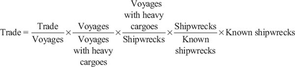
This long equation expresses an illuminating tautology. It shows the volume of trade, called simply “Trade” in the equation, as the product of a series of ratios. If you cancel all the magnitudes that appear in both the denominator and numerator of a ratio, the equation says only that the volume of trade equals the volume of trade. The shipwreck index is a good indicator of trade only if all the ratios in the equation stay constant. If we suspect they were not constant, the equation allows us to structure our investigation of changes in pursuit of a better index of trade.
For example, the ratio of voyages to those with heavy cargoes can change for many reasons. The most obvious is the nature of containers. Amphoras are heavy and durable. Ships containing amphoras will sink, and the amphoras will stay intact even as the ships themselves disappear. Late Romans learned to use barrels instead of amphoras to ship liquids. This was a gain to the porters who carried these containers, but it was a loss to archaeologists who could not recover evidence of barrel shipments. A rise in the ratio of total voyages to those containing heavy amphoras will change the ratio of known shipwrecks to the volume of trade. Put differently, a decline in the number of known shipwrecks might be an index of a decline in trade or of technological progress that reduced the dead weight being carried around in the form of amphoras. The shipwreck index may be a more accurate indicator of trade volumes during its rise in the Roman Republic than it is during its decline during the Roman Empire.
The ratio of voyages with heavy cargoes to shipwrecks is affected by the skill of ship captains. If the captains learned how to improve their navigation or weather prediction, this ratio might have changed. The ratio of shipwrecks to known shipwrecks similarly is affected by the skill of archaeologists in dating shipwrecks. McCormick (forthcoming) reported progress in this dimension, arguing that we now can date shipwrecks previous generations could not.
Wilson (2009a) argued that the indexes that Scheidel (2009a) used to date Roman economic growth were too fragile to bear this weight. He discussed the problems with the shipwreck data just noted and compared the overall index with an index of shipwrecks carrying stone cargoes. This rough device to correct for the bias in the index provided a different time path for the relevant wrecks. Other proxies were similarly flawed or ambiguous, and Wilson argued that the sum of the evidence was inconclusive. He concluded, “The apparent convergence of the proxies is very misleading” (Wilson 2009a, 71).
It is likely that both processes were in operation in the early Roman Empire. More evidence may produce a more precise accounting, but there does not seem to be evidence as yet or agreement that hypothesis one or two is correct while the other is wrong. Economists create these oppositions for intellectual clarity, but history has a way of splitting the difference or revealing a more complex story than either extreme hypothesis. At this stage, it is clear that there was a one-time gain from comparative advantage as the Romans promoted Mediterranean trade (see chapter 2). A unified Mediterranean market promoted regional specialization and associated income gains. There also were improvements in the technologies of agriculture and other economic activities. Wilson reminds of us of what we might call “hard” technologies that leave archaeological remains. To that should be added the “soft” technologies of attitudes and markets described in previous chapters that also contributed to economic prosperity and growth. We do not know the full distribution of these changes or the timing of their spread, but it is clear that much more was going on than simply unifying the Mediterranean world.
Whichever hypothesis is more correct, neither of them implies that economic growth could have continued from Roman times until today. Without industrialization, the Malthusian constraints described in the model of this chapter still held. They held loosely, allowing centuries of economic growth under favorable conditions, but they eventually would constrain this growth. The question therefore is not whether Malthusian constraints were present, but rather what changes in Roman times led to growth within these constraints and how far growth went. There were many shocks in the early centuries of this era, from the Antonine Plague to inflation, political instability, and invasions (see chapter 4). The purpose of this simple Malthusian model and the discussion it has generated is to clarify the complex interactions between these historical events.
We know that England began to industrialize in the late eighteenth century and that the English innovations spread throughout Western Europe in the nineteenth century. Why didn’t a similar process happen in ancient times? The Malthusian model described here cannot answer such a complex question, and no answer will be forthcoming here. The model lets us understand what is similar and different in the two periods, sharpening the question. A more detailed model of technological change then is needed to compare ancient Rome and early modern England.
As described earlier, technological change can expand the resource constraint and allow both population and per capita incomes to rise. If technological change continues for a while, incomes can remain high while population rises. There are two reasons why population continues to rise. The technological change continues to shift outward the resource constraint, as seen in figure 10.4, which allows population and income to increase. In the short run, income increases, which then allows births to exceed deaths, which is how population increases. These two mechanisms can provide a stable situation where incomes are higher than Malthusian subsistence, y*, and population is growing. The change from a static resource constraint to an expanding one has resulted in the growth of per capita incomes from y* to its new level, accompanied by population growth.
A constant rate of technological progress therefore leads only to limited economic growth. Growth becomes a transitory phenomenon as the economy moves from a static Malthusian equilibrium to a dynamic one based on continuing technical change. This appears to describe the growth in real wages observed in preindustrial London and Amsterdam as the growth of trade in the seventeenth and eighteenth centuries expanded the English and Dutch resource constraint. Real wages in most European cities fell in this time as population grew, but not in these progressive cities. By the eighteenth century the difference between the high-wage cities and the low-wage cities on the European continent was about two-to-one (Allen 2001).
A small modification of the Malthusian model allows it to incorporate continuing economic growth. Instead of assuming that the rate of expansion of the resource constraint is constant, assume that it is proportional to the size of the population. In other words, the rate of technological progress rises when population rises. This is the assumption used by Kremer (1993) in his analysis of population growth for the last million years, by Diamond (1997) in his description of how the Neolithic Revolution set the stage for the Industrial Revolution, and by Galor (2011) in his presentation of his unified growth theory. I show in an appendix to this chapter that this assumption allows incomes and population to rise indefinitely.
This process describes the path of the Industrial Revolution. Technological improvement started to accelerate in the late eighteenth century and continued to increase as population also increased. Later, about a century after the start of industrialization, the rate of population growth diminished as the Demographic Transition took place. Women who had education could see the value of education for their children in the increasingly industrial world. They opted to have “better” children, that is, children with education and therefore “human capital,” in place of having more children. In this context, the Malthusian model no longer provides many insights into the paths of industrial societies, as described in chapter 9.
This avenue was not open to Rome, at least not in the form that the Industrial Revolution of the eighteenth century took place. Allen (2009b) showed that industrialization began in England as a result of two forces. The first was high wages. Both England and the Dutch Republic had high wages as a result of their profits from international trade. Roman Italy shared this prosperity two millennia earlier as a result of war booty and the profits from Mediterranean trade, but only England had the Industrial Revolution. Allen argued that high wages needed to be coupled with cheap power to generate industry. The coal industry of England shipped coal from the west and north of England to London. The price of fuel in London was about the same as in other advanced economies, but the price of fuel closer to the source was uniquely low. It was “the cheapest energy in the world” (Allen 2009b, 97).
The uniquely high ratio of wages to power costs gave rise to the Industrial Revolution, not only in England, but in only a specific part of England. Steam engines and iron technology improved in the north and west of England where coal was dirt cheap. The high ratio of wages to energy costs allowed England to produce goods that were competitive with goods produced elsewhere in Europe despite the high English wages. It explains why the first industrialization took place in England rather than in Holland or France. “The cheap energy economy was a foundation of Britain’s economic success. Inexpensive coal provided the incentive to invent the steam engine and metallurgical technology of the Industrial Revolution” (Allen 2009b, 104).
The high ratio of wages to energy costs was not only absent in eighteenth-century continental Europe; it was absent as well in the Roman Empire. Despite the technical progress being made then that we are discovering more about, there was no possibility of escaping from the Malthusian constraints with the price ratios that existed then. However prosperous Rome may have been, it was not on the verge of having an Industrial Revolution. There was no analog of the British coal industry in antiquity and therefore no possibility that industrialization could have begun in the ancient world.
Even under hypothesis one, Romans in the early empire appear to have been living well. If this improvement came from the increase in trade, then the residents of Roman Italy may have been similar to the English and Dutch in the seventeenth and eighteenth centuries. Allen (2003) showed that the rise in Atlantic trade increased real wages in those countries before industrialization. Trade did the same for Roman Italy, and it may also, following Ricardo’s analysis, have raised real wages elsewhere in the early Roman Empire. I pursue this further in chapter 11.
Any model is a simplification, and the one explained in this chapter is no exception. The exposition here does not aim to capture all the details of this economic expansion. Instead it provides a framework in which the details that emerge from various kinds of research can fit. It provides a mechanism to turn the odd facts gathered by archaeologists into a coherent picture. With more information, perhaps stimulated by having such a framework, we can aspire to constructing a more detailed model. A recent book stated, “Ancient economic history remains a largely undertheorized field of study” (Banaji 2001). I filled a small part of this lack by analyzing a simple Malthusian model. The model is designed to explain how per capita incomes could have grown in a predominantly Malthusian world. This is not possible in equilibrium, and this paper is about the behavior of this model out of the well-known Malthusian equilibrium.
There are several benefits of using a model like this one. Most important, it allows us to integrate recent archaeological discoveries about Roman technology into a coherent view of the Roman economy. It helps us resolve an apparent conflict between the observations we are accumulating about the good life of ordinary Roman citizens or at least structure our disagreements (Scheidel 2009a; Wilson 2009a).
The model also allows us to engage in a structured discussion of alternative histories, what economic historians of the modern world call counterfactuals. What would have happened if the western Roman Empire had not collapsed? We will never know. This model allows us to speculate in a coherent way about what might have been. The comparison with the Industrial Revolution showed an alternative history—about a far different time and place. It is clear that Rome could not have gone that way even if various other factors had been different. The Malthusian model will not help us identify which of those other factors were more important than others; it will help us understand the consequences of economic decline.
Even this simple model helps define questions for Roman archaeology. Hypothesis one above is that there was a single spurt of productivity change whose effects were gradually eroded by Malthusian pressures. Hypothesis two is that Roman productivity growth continued until some unrelated factors inhibited it, allowing living standards to stay high for a longer period. We need more detailed evidence than now exists to make this differentiation.
Finally, the use of this kind of model provides a bridge to help unify the study of ancient and more modern history. At the very least, it can integrate the analysis of ancient plagues with that of more modern ones. It can help us redraw graphs like the one shown in figure 10.1 to reveal accomplishments of people who lived long ago that have been largely forgotten by modern historians. And it raises questions about modern history as much as about ancient history. For all of the factors that doomed the Roman Empire must have been missing or at least modified two millennia later when the Industrial Revolution took place. A model that structures our discussion allows us to place ancient economic history into the general study of economic history.