It must be understood, however, that α(), β() do not disclose which strategy of the opponent will inflict this (maximum) loss upon the player who is using or . It is, in particular, not at all certain that if the opponent uses some particular good strategy, i.e. an ₀ in or a ₀ in Ā, this in itself implies the maximum loss in question. If a (not good) or is used by the player, then the maximum loss will occur for those if of the opponent, for which

i.e. if is optimal against the given optimal against the given . And we have never ascertained whether any fixed ₀ or ₀ can be optimal against all or .

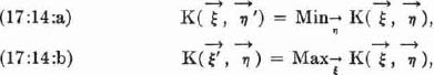
17.10.2. Let us therefore call an which is optimal against all or —i.e. which fulfills (17:14:a), or (17:14:b) in 17.10.1. for all , —permanently optimal. Any permanently optimal is necessarily good; this should be clear conceptually and an exact proof is easy.³ But the question remains: Are all good strategies also permanently optimal? And even: Do any permanently optimal strategies exist?

In general the answer is no. Thus in Matching Pennies or in Stone, Paper, Scissors, the only good strategy (for player 1 as well as for player 2) is respectively.1 If player 1 played differently—e.g. always “heads”² or always “stone”²—then he would lose if the opponent countered by playing “tails”³ or “paper.”³ But then the opponent’s strategy is not good—i.e. respectively—either. If the opponent played the good strategy, then the player’s mistake would not matter.⁴

We shall get another example of this—in a more subtle and complicated way—in connection with Poker and the necessity of “bluffing,” in 19.2 and 19.10.3.

All this may be summed up by saying that while our good strategies are perfect from the defensive point of view, they will (in general) not get the maximum out of the opponent’s (possible) mistakes,—i.e. they are not calculated for the offensive.

It should be remembered, however, that our deductions of 17.8. are nevertheless cogent; i.e. a theory of the offensive, in this sense, is not possible without essentially new ideas. The reader who is reluctant to accept this, ought to visualize the situation in Matching Pennies or in Stone, Paper, Scissors once more; the extreme simplicity of these two games makes the decisive points particularly clear.

Another caveat against overemphasizing this point is: A great deal goes, in common parlance, under the name of “offensive,” which is not at all “offensive” in the above sense,—i.e. which is fully covered by our present theory. This holds for all games in which perfect information prevails, as will be seen in 17.10.3.⁵ Also such typically “aggressive” operations (and which are necessitated by imperfect information) as “bluffing” in Poker.⁶

17.10.3. We conclude by remarking that there is an important class of (zero-sum two-person) games in which permanently optimal strategies exist. These are the games in which perfect information prevails, which we analyzed in 15. and particularly in 15.3.2., 15.6., 15.7. Indeed, a small modification of the proof of special strict determinateness of these games, as given loc. cit., would suffice to establish this assertion too. It would give permanently optimal pure strategies. But we do not enter upon these considerations here.

Since the games in which perfect information prevails are always specially strictly determined (cf. above), one may suspect a more fundamental connection between specially strictly determined games and those in which permanently optimal strategies exist (for both players). We do not intend to discuss these things here any further, but mention the following facts which are relevant in this connection:

(17:G:a)	It can be shown that if permanently optimal strategies exist (for both players) then the game must be specially strictly determined.
(17:G:b)	It can be shown that the converse of (17:G:a) is not true.
(17:G:c)	Certain refinements of the concept of special strict determinateness seem to bear a closer relationship to the existence of permanently optimal strategies.

17.11. The Interchange of Players. Symmetry

17.11.1. Let us consider the role of symmetry, or more generally the effects of interchanging the players 1 and 2 in the game Γ. This will naturally be a continuation of the analysis of 14.6.

As was pointed out there, this interchange of the players replaces the function (τ₁, τ₂) by –(τ₂, τ₁). The formula (17:2) of 17.4.1. and 17.0. shows that the effect of this for K(, ) is to replace it by – K(, ). In the terminology of 16.4.2., we replace the matrix (of (τ₁, τ₂) cf. 14.1.3.) by its negative transposed matrix.

Thus the perfect analogy of the considerations in 14. continues; again we have the same formal results as there, provided that we replace (Cf. the previous occurrence of this in 17.4. and 17.8.)

We saw in 14.6. that this replacement of (τ₁, τ₂) by –(τ₂, τ₁) carries v₁, v₂ into –v₂, –v₁. A literal repetition of those considerations shows now that the corresponding replacement of K(, ) by –K (, ) carries into –v₂, –v₁. Summing up: Interchanging the players 1, 2, carries v₁, v₂, into –v₂, –v₁, –, –,.

The result of 14.6. established for (special) strict determinateness was that v = v₁ = v₂ is carried into –v = –v₁ = –v₂. In the absence of that property no such refinement of the assertion was possible.

At the present we know that we always have general strict determinateness, so that Consequently this is carried into

Verbally the content of this result is clear: Since we succeeded in defining a satisfactory concept of the value of a play of Γ (for the player 1), v′, it is only reasonable that this quantity should change its sign when the roles of the players are interchanged.

17.11.2. We can also state rigorously when the game Γ is symmetric. This is the case when the two players 1 and 2 have precisely the same role in it,—i.e. if the game Γ is identical with that game which obtains from it by interchanging the two players 1, 2. According to what was said above, this means that

or equivalently that

This property of the matrix (τ₁, τ₂) or of the bilinear form K (, ) was introduced in 16.4.4, and called skew-symmetry.1,2

In this case v₁, v₂ must coincide with –v₂, –v₁; hence v₁ = –v₂, and since v₁ v₂, so v₁ 0. But v′ must coincide with –v′; therefore we can even assert that

v′ = 0.³

So we see: The value of each play of a symmetrical game is zero.

It should be noted that the value v′ of each play of a game Γ could be zero without Γ being symmetric. A game in which v′ = 0 will be called fair.

The examples of 14.7.2., 14.7.3. illustrate this: Stone, Paper, Scissors is symmetric (and hence fair); Matching Pennies is fair (cf. 17.1.) without being symmetric.⁴

In a symmetrical game the sets Ā, of (17:B:a), (17:B:b) in 17.8. are obviously identical. Since Ā = we may put = in the final criterion (17:D) of 17.9. We restate it for this case:

(17:H)

In a symmetrical game, belongs to Ā if and only if this is true: For each τ2 = 1, · · · β2 for which does not assume its minimum (in τ2) we have

Using the terminology of the concluding remark of 17.9., we see that the above condition expresses this: is optimal against itself.

17.11.3. The results of 17.11.1., 17.11.2.—that in every symmetrical game v′ = 0—can be combined with (17:C:d) in 17.8. Then we obtain this:

(17:I)

In a symmetrical game each player can, by playing appropriately, avoid loss1 irrespective of what the opponent does.

We can state this mathematically as follows:

If the matrix (τ₁, τ₂) is skew-symmetric, then there exists a vector in with

This could also have been obtained directly, because it coincides with the last result (16:G) in 16.4.4. To see this it suffices to introduce there our present notations: Replace the i, j, a(i, j) there by our τ₁, τ₂, (τ₁, τ₂) and the there by our .

It is even possible to base our entire theory on this fact, i.e. to derive the theorem of 17.6. from the above result. In other words: The general strict determinateness of all Γ can be derived from that one of the symmetric ones. The proof has a certain interest of its own, but we shall not discuss it here since the derivation of 17.6. is more direct.

The possibility of protecting oneself against loss (in a symmetric game) exists only due to our use of the mixed strategies , (cf. the end of 17.7.). If the players are restricted to pure strategies τ₁, τ₂ then the danger of having one’s strategy found out, and consequently of sustaining losses, exists. To see this it suffices to recall what we found concerning Stone, Paper, Scissors (cf. 14.7. and 17.1.1.). We shall recognize the same fact in connection with Poker and the necessity of “bluffing” in 19.2.1.

1 Cf. (11:D:a), (11:D:b) at the end of 11.2.3. We suppress the index 1.

² Then (τ) = 0, cf. 11.4.

³ The existing “double solitaires” are competitive games between the two participants, i.e. two-person games.

⁴ The individual members themselves cannot be considered as players, since all possibilities of conflict among them, as well as coalitions of some of them against the others, are excluded.

¹ We do not in the least intend, of course, to detract from the enormous importance of those discoveries. It is just because of their great power that we are now in a position to treat this side of the matter as briefly as we do. We are interested in those aspects of the problem which are not settled by the concept of probability alone; consequently these and not the satisfactorily settled ones must occupy our attention.

² Concerning the important connection between the use of mathematical expectation and the concept of numerical utility, cf. 3.7. and the considerations which precede it.

³ Some games like Roulette are of an even more peculiar character. In Roulette the mathematical expectation of the players is clearly negative. Thus the motives for participating in that game cannot be understood if one identifies the monetary return with utility.

¹ Although they do not appear in the above canonical forms (x), (x, y).

² We could also treat k in (d) and k in (e) like k in (c), i.e. as a variable.

¹ The concept of a function is closely allied to that of a set, and the above should be viewed in parallel with the exposition of 8.2.

² Proof: Consider two such x₀, say and . Then and . Hence .

¹ E.g. if (x) ≡ x with all real numbers as domain, then neither Max (x) nor Min (x) exist.

² Typical examples: The functions _k(τ₁, · · · , τ_n) of 11.2.3. (or of (e) in 13.1.2.), the function (τ₁, τ₂) of 14.1.1.

³ Typical examples: The functions in 17.4., the functions in 17.5.2. The variables of all these functions are or or both, with respect to which subsequent maxima and minima are formed.

Another instance is discussed in 46.2.1. espec. footnote 1 on p. 384, where the mathematical background of this subject and its literature are considered. It seems unnecessary to enter upon these here, since the above examples are entirely elementary.

¹ Of course Max (a, b, · · · ) [Min (a, b, · · · )] is simply the greatest [smallest] one among the numbers a, b, · · · .

² A well known operation in analysis which kills a variable τ is the definite integral: (x) is a function of x, but is a constant.

³ We treated y, z, · · · as constant parameters in 13.2.2. But now that x has been killed we release the variables y, z, · · · .

⁴ Observe that if two or more operations are applied, the innermost applies first and kills its variable; then the next one follows suit, etc.

⁵ With one variable less, since these operations kill one variable each.

⁶ Further variables of , if any, may be treated as constants for the purpose of this analysis.

¹ The combination Min_x Max_y requires no treatment of its own, since it obtains from the above—Max_x Min_y—by interchanging x, y.

¹ All this is closely connected with—although not precisely a special case of—certain more general mathematical theories involving extremal problems, calculus of variations, etc. Cf. M. Morse: The Critical Points of Functions and the Calculus of Variations in the Large, Bull. Am. Math. Society, Jan.–Feb. 1929, pp. 38 cont., and What is Analysis in the Large? Am. Math. Monthly, Vol. XLIX, 1942, pp. 358 cont.

² This follows from (13:C*) in 13.5.2. There exists an equally simple direct proof: Consider two saddle points x₀, y₀, say Then:

,

i.e.: Similarly
Hence

³ Clearly the operation Sa_x/y(x, y) kills both variables x, y. Cf. 13.2.3.

¹ Only under our hypothesis at the beginning of this section! Otherwise there exist no saddle points at all.

² If the x, y are positive integers, then this can certainly be brought about by two appropriate permutations of their domain.

³ The general mathematical concepts alluded to in footnote 1 on p. 95 are free from these limitations. They correspond precisely to the everyday idea of a pass.

⁴ The reader is asked to visualize this: Although itself a function, f may perfectly well be the variable of another function.

¹ Cf. (11:D) in 11.2.3.

¹ The domain, of course, is prescribed: It consists of all pairs τ₁, τ₂ with τ₁ = 1,  · · · , β₁; τ₂ = 1, · · · , β₂. This is a finite set, so all Max and Min exist, cf. the end of 13.2.1.

¹ The point is, of course, that this is not a tug-of-war. The two players have opposite interests, but the means by which they have to promote them are not in opposition to each other. On the contrary, these “means”—i.e. the choices of τ₁, τ₂—are apparently independent. This discrepancy characterizes the entire problem.

² Thus Γ₁—while extremely simple—is no longer in the normalized form.

³ Thus Γ₂—while extremely simple—is no longer in the normalized form.

⁴ Of course, to be precise we should say “less than or equal to” instead of “less,” and “more than or equal to” instead of “more.”

¹ Observe that τ₂ may not be uniquely determined: For a given τ₁ the τ₂-function (τ₁, τ₂) may assume its τ₂-minimum for several values of τ₂. The value of (τ₁, τ₂) will, however, be the same for all these τ₂, namely the uniquely defined minimum value Min_τ2 (τ₁, τ₂). (Cf. 13.2.1.)

² For the same reason as in footnote 1 above, the value of τ₁ may not be unique, but the value of Min_τ2 (τ₁, τ₂) is the same for all τ₁ in question, namely the uniquely-defined maximum value

³ 2 is informed of the value of τ₁ when called upon to make his choice of τ₂,—this is the rule of Γ₁. It follows from our concept of a strategy (cf. 4.1.2. and end of 11.1.1.) that at this point a rule must be provided for 2’s choice of τ₂ for every value of τ₁,—irrespective of whether 1 has played well or not, i.e. whether or not the value chosen belongs to A.

⁴ In all, this τ₁ is treated as a known parameter on which everything depends,—including the set B_τ1 from which τ₂ ought to be chosen.

¹ Recall that τ₁ must be chosen without knowledge of τ₂, while τ₂ is chosen in full knowledge of τ₁.

¹ 1 is informed of the value of τ₂ when called upon to make his choice of τ₁—this is the rule of Γ₂ (Cf. footnote 3 on p. 101).

² In all this τ₂ is treated as a known parameter on which everything depends, including the set A_τ2 from which τ₁ ought to be chosen.

³ Remember that τ₂ must be chosen without any knowledge of τ₁, while τ₁ is chosen with full knowledge of τ₂.

¹ Observe that the original game Γ was symmetric with respect to the two players 1 and 2, if we let each player take his function ₁(τ₁, τ₂), ₂(τ₁, τ₂) with him in an interchange; i.e. the personal moves of 1 and 2 had both the same character in Γ.

For a narrower concept of symmetry, where the functions ₁(τ₁, τ₂), ₂(τ₁, τ₂) are held fixed, cf. 14.6.

² This point deserves careful consideration: Naturally these two characterizations must obtain from each other by interchanging the roles of the players 1 and 2. But in this case the statements coincide also directly when no interchange of the players is made at all. This is due to their individual symmetry.

¹ For player 2 the values are consequently –v₁, –v₂.

² In the game Γ—which is in the normalized form—the strategy is just the actual choice at the unique personal move of the player. Remember how this normalized form was derived from the original extensive form of the game; consequently it appears that this choice corresponds equally to the strategy in the original game.

³ For an interpretation of all these assumptions, cf. 17.3.1.

¹ Observe that this expression for the advantage in question applies for both players: The advantage for the player 1 is v₂ – v₁; for the player 2 it is (–v₁) – (–v₂) and these two expressions are equal to each other, i.e. to Δ.

¹ Since this is the game Γ each player must make his choice (of τ₁ or τ₂) without knowledge of the other player’s choice (of τ₂ or τ₁). Contrast this with (14:A:b) in 14.3.1. for Γ₁ and with (14:B:b) in 14.3.3. for Γ₂.

¹ This is no longer the operation of interchanging the players used in 14.3.4. There we were only interested in the arrangement and the state of information at each move, and the players 1 and 2 were considered as taking their functions ₁(τ₁, τ₂) and ₂(τ₁, τ₂) with them (cf. footnote 1 on p. 104). In this sense Γ was symmetric, i.e. unaffected by that interchange (id.).

At present we interchange the roles of the players 1 and 2 completely, even in their functions (τ₁, τ₂) and (τ₁, τ₂).

² We had to interchange the variables τ₁, τ₂ since τ₁ represents the choice of player 1 and τ₂ the choice of player 2. Consequently it is now τ₂ which has the domain 1, · · · , β₁. Thus it is again true for _k(τ₂, τ₁)—as it was before for _k(τ₁, τ₂)—that the variable before the comma has the domain 1, · · · , β₁ and the variable after the comma, the domain 1, · · · , β₂.

³ This is a mere change of notations: The variables τ₁, τ₂ are changed around to τ₂, τ₁.

4 This is in harmony with footnote 1 on p. 105, as it should be.

¹ This is in harmony with footnote 1 on p. 106, as it should be.

² Cf. however, 17.8.1.

³ In plainer language: Δ > 0 means that it is not possible in this game for each player simultaneously to be cleverer than his opponent. Consequently it seems desirable to know just how clever each particular player is.

¹ “Paper covers the stone, scissors cut the paper, stone grinds the scissors.”

² As mentioned before, we shall show in 17.1. that it can be done.

¹ I.e. have ν – 1 instead of ν. Repeated application of this “inductive” step—if feasible at all—will reduce the game Γ to one with 0 steps; i.e. to one of fixed, unalterable outcome. And this means, of course, a complete solution for Γ. (Cf. (15;C:a) in 15.6.1.)

² E.g. Γ is the game of Chess, and ₁ a particular opening move—i.e. choice at ₁—of “white,” i.e. player 1. Then Γ₁ is again Chess, but beginning with a move of the character of the second move in ordinary Chess—a “black,” player 2—and in the position created by the “opening move” ₁. This dictated “opening move” may, but need not, be a conventional one (like E2-E4).

The same operation is exemplified by forms of Tournament Bridge where the “umpires” assign the players definite—known and previously selected—“hands.” (This is done, e.g., in Duplicate Bridge.)

In the first example, the dictated move ₁ was originally personal (of “white,” player 1); in the second example it was originally chance (the “deal”).

In some games occasionally “handicaps” are used which amount to one or more such operations.

³ We should really use the indices 1, · · · , ν – 1 and indicate the dependence on ₁; e.g. by writing But we prefer the simpler notation ₂, · · · , _ν.

⁴ This is the terminology of 6.3.; i.e. we use the special form of dependence in the sense of 7.2.1. Using the general description of 7.2.1. we must state (15:A:a) like this: For every personal move _κ, κ = 2, · · · , ν, the set Φ_κ, contains the function in σ₁.

¹ This ₁ is an exception from (8:B:a) in 8.3.1.; cf. the remark concerning this (8:B:a) in footnote 1 on p. 63, and also footnote 4 on p. 69.

² Proof: Ω belongs to ₁, which is a subpartition of ₁; hence Ω is a subset of an element of ₁. This element is necessarily equal to Ω. All other elements of ₁ are therefore disjunct from Ω (cf. 8.3.1.), i.e. empty.

³ ₁, ₁(k₁) unlike ₁ (cf. above) must fulfill both (8:B:a), (8:B:b) in 8.3.1.; hence both have no further elements besides Ω.

⁴ They represent the alternatives ₁(1), · · · , ₁(α₁) of 6.2. and 9.1.4., 9.1.5.

¹ We do not wish to change the enumeration to κ = 1, · · · , v – 1, cf. footnote 3 on p. 113.

² _κ represents the umpire’s state of information, but this is an objective fact: the events up to that moment have determined the course of the play precisely to that extent (cf. 9.1.2.).

³ Namely, giving him additional information.

¹ ₁ = 1, · · · , α₁; ₂ = 1, · · · , α₂ where α₂ = α₂(₁); ₃ = 1, · · · , α₃ where α₃ = α₃(₁, ₂); etc., etc.

¹ We stated this above for λ = 2, 3, · · · ; for λ = 1 it is automatically true: every partition is a subpartition of ₁ since ₁ consists of the one set Ω ((10:1:f) in 10.1.1.).

² For the motivation—if one is wanted—cf. the argument of footnote 3 on p. 63.

³ From now on we write σ₁, σ₂, · · · , σ_v instead of ₁, ₂, · · · , _v because no misunderstandings will be possible.

¹ This is clear intuitively. The reader may verify it from the formalistic point of view by applying the definitions of 11.1.1. and (11:A) in 11.1.3. to the situation described in 15.2.1.

¹ This is merely a heuristic argument, since the principles on which the “solutions” of 14.3.1., 14.3.3. are based are not entirely the same as those by which we disposed of the strictly determined case in 14.5.1., 14.5.2., although the former principles were a stepping stone to the latter. It is true that the argument could be made pretty convincing by an “unmathematical,” purely verbal, amplification. We prefer to settle the matter mathematically, the reasons being the same as given in a similar situation in 14.3.2.

² This is clear intuitively. The reader may verify it from the formalistic point of view, by reformulating the definition of Γ₁ as given in 14.2. in the partition and set terminology, and then applying the definitions of 11.1.1. and (11:A) in 11.1.3.

The essential fact is, at any rate, that in Γ₁ the personal move of player 1 is preliminary to that of player 2.

³ Cf. footnote 1 on p. 118 or footnote 2 above.

¹ Cf. footnote 1 on p. 118 or footnote 2 on p. 120.

² must be treated in this case as a constant.

This step is of course a rather trivial one,—cf. the argument loc. cit.

³ In contrast to 15.4.2., there is now an essential difference between the treatments of v₁ and v₂.

⁴ is killed in this case by the operation Max.

This step is not trivial. It makes use of (13:E) in 13.5.3., i.e. of the essential result of that paragraph, as stated in 15.4.3.

¹ Cf. the game in footnote 2 on p. 76 or in 15.3.1. In the partition and set terminology: For v = 0 (10:1:f), (10:1:g) in 10.1.1. show that Ω has only one element, say So play the role indicated above.

² I.e. each player has only one strategy, which consists of doing nothing.

³ This is, of course, rather obvious. The essential step is (15:C:b).

⁴ I.e. the fact mentioned at the end of 15.5.3., that the formula is the same for k = 1,2 for each value of k₁.

⁵ Cf. footnote 3 on p. 117.

¹ Cf. the remarks concerning in 15.3.1.

² Cf. (15:C:a) in 15.6.1., particularly footnote 1 on p. 123.

³ This is due mainly to the enormous value of v. For Chess, cf. the pertinent part of footnote 3 on p. 59. (The v* there is our v, cf. the end of 7.2.3.)

¹ This is the simplest way to interpret a “win,” “tie,” or “loss” of a play by the player k.

² Every value of is one of _k; every value of _k—in the absence of chance moves—is one of , cf. loc. cit. If there were chance moves, then the value of _k would be the probability of a “win” minus that of a “loss,” i.e. a number which may lie anywhere between 1 and –1.

³ When there are chance moves, then (τ₁, τ₂) is the excess probability of a “win” over a “loss,” cf. footnote 2 above. The players try to maximize or to minimize this number, and the sharp trichotomy of (15:D:a)—(15:D:c) above does not, in general, obtain.

Although Backgammon is a game in which complete information prevails, and which contains chance moves, it is not a good example for the above possibility: Backgammon is played for varying payments, and not for simple “win,” “tie” or “loss,”—i.e. the values of the _k are not restricted to the numbers 1, 0, –1.

¹ In imagining the application of this procedure to any specific game it must be remembered that we assume the length v of Γ to be fixed. If v is actually variable—and it is so in most games (cf. footnote 3 on p. 58)—then we must first make it constant, by the device of adding ”dummy moves” to Γ as described at the end of 7.2.3. It is only after this has been done that the above regression through _v, _v–1, · · · , ₁ becomes feasible.

For practical construction this procedure is of course no better than that of 15.4.-15.6.

Possibly some very simple games, like Tit-tat-toe, could be effectively treated in either manner.

¹ This is not necessarily true if the sum is not constantly zero, or if there are more than two players. For details cf. 20.1., 24.2.2., 58.3.

² Cf. in this respect particularly (14:D:a), (14:D:b), (14:C:d), (14:C:e) in 14.5.1. and (14:C:a), (14:C:b) in 14.5.2.

³ Cf. T. Bonessen and W. Fenchel: Theorie der konvexen Körper, in Ergebnisse der Mathematik und ihrer Grenzgebiete, Vol. III/1, Berlin 1934. Further investigations in H. Weyl: Elementare Theorie der konvexen Polyeder. Commentarii Mathematici Helvetic, Vol. VII, 1935, pp. 290–306.

¹ I.e. the n-uplets {x₁, · · · , x_n} are not merely sets in the sense of 8.2.1. The effective enumeration of the x_i by means of the index i = 1, · · · , n is just as essential as the aggregate of their values. Cf. the similar situation in footnote 4 on p. 69.

² Much in modern analysis tends to corroborate this attitude.

³ This at least is the orthodox geometrical standpoint.

⁴ Thus the zero vector has all components 0, while the coordinate vectors have all components but one 0—that one component being 1, and its index j for the j-th coordinate vector.

5 δ_ij is the “symbol of Kronecker and Weierstrass,” which is quite useful in many respect.

1 The x_j are numbers, and hence they act in as scalar multipliers. is a vector summation.

2 For n = 3, i.e. in ordinary (3-dimensional Euclidean) space, these are just the ordinary (2-dimensional) planes. In our general case they are the ((n – 1)-dimensional) analogues; hence the name.

¹ The Euclidean—Pythagorean—meaning of these notions is immediate.

² For the reader who is familiar with topology, we add: To be exact, this sentence should be qualified—the statement is meant for closed convex sets. This guarantees the existence of the minimum that we use in the proof that follows. Regarding these concepts, cf. footnote¹ on page 384.

¹ > 0 and not only 0. Indeed, = 0 would necessitate x₁ = · · · = x_m = 0 which is impossible since

¹ The two alternatives (16:19:a), (16:19:b) do not exclude each other: Their conjunction ie precisely (16:18:c).

² This result could also have been obtained directly from the final result of 16.4.1.: (16:19:a) is precisely (16:16:a) there, and (16:19:b) is a weakened form of (16:16:b) there. We gave the above more detailed discussion because it gives a better insight into the entire situation.

¹ E.g. he could throw a die—of course without letting the opponent see the result—and then play “tails” if the number of spots showing is even, and “heads” if that number is odd.

² I.e. his probability of winning equals his probability of losing, because under these conditions the probability of matching as well as that of not matching will be , whatever the opponent’s conduct.

³ Say p, 1 – p. For the player himself we used the probabilities , .

⁴ All this, of course, in the statistical sense: that the player cannot lose, means that his probability of losing is his probability of winning. That he cannot win, means that the former is to the latter. Actually each play will be won or lost, since Matching Pennies knows no ties.

⁵ We mean specifically (14:C:d), (14:C:e) in 14.5.1.

⁶ A chance device could be introduced as before. The die mentioned in footnote 1, above, would be a possible one. E.g. the player could decide “stone” if 1 or 2 spots show, “paper” is 3 or 4 spots show, “scissors” if 5 or 6 show.

¹ In Stone, Paper, Scissors there exists a tie, but no loss still means that the probability of losing is the probability of winning, and no gain means the reverse. Cf. footnote 4 on p. 144.

² That these probabilities were the same for all strategies (, or , , in the examples of the last paragraph) was, of course accidental. It is to be expected that this equality was due to the symmetric way in which the various alternatives appeared in those games. We proceed now on the assumption that the appearance of probabilities in formulating a strategy was the essential thing, while the particular values were accidental.

³ The Δ > 0 of 14.7.1.

¹ But not necessarily the only one.

² If the opponent has enough statistical experience about the player’s “style,” or if he is very shrewd in rationalizing his expected behavior, he may discover the probabilities—frequencies—of the various strategies. (We need not discuss whether and how this may happen. Cf. the argument of 17.3.1.) But by the very concept of probability and randomness nobody under any conditions can foresee what will actually happen in any particular case. (Exception must be made for such probabilities as may vanish; cf. below.)

3 In this case he clearly increases the danger of having his strategy found out by the opponent. But it may be that the strategy or strategies in question have such intrinsic advantages over the others as to make this worth while. This happens,—e.g. in an extreme form for the “good” strategies of the strictly determined case (cf. 14.5., particularly (14:C:a), (14:C:b) in 14.5.2.).

¹ I.e. “gradual,” “successive” observations of the behavior of the opponent within one play.

² Our method is, of course, the empirical one: We are trying to understand, formalize and generalize those features of the simplest games which impress us as typical. This is, after all, the standard method of all sciences with an empirical basis.

3 This is full cognizance of the fact that we do not (yet) possess one, and that we cannot imagine (yet) what it would be like, if we hail one.

All this is—in its own domain—no worse than any other indirect proof in any part of science (e.g. the per absurdum proofs in mathematics and in physics).

¹ There are several important examples of this performance in physics. The successive approaches to Special and to General Relativity or to Wave Mechanics may be viewed as such. Cf. A. D’ Abro: The Decline of Mechanism in Modern Physics, New York 1939.

² This too occurs in physics. The N. Bohr-Heisenberg analysis of “quantities which are not simultaneously observable” in Quantum Mechanics permits this interpretation. Cf. N. Bohr: Atomic Theory and the Description of Nature, Cambridge 1934 and P.A.M. Dirac: The Principles of Quantum Mechanics, London 1931, Chap. I.

³ Why it would be unwise not to follow it is none of our concern at present; we have assumed that the theory is absolutely convincing.

That this is not impossible will appear from our final result. We shall find a theory which is satisfactory; nevertheless it implies that the player’s strategy is found out by his opponent. But the theory gives him the directions which permit him to adjust himself so that this causes no loss. (Cf. the theorem of 17.6. and the discussion of our complete solution in 17.8.)

⁴ I.e. a theory using our present devices only. Of course we do not pretend to be able to make “absolute” statements. If our present requirements should turn out to be unfulfillable we should have to look for another basis for a theory. We have actually done this once by passing from 14. (with pure strategies) to 17. (with mixed strategies).

5 The indirect argument, as outlined above, gives only necessary conditions. Hence it may establish absurdity (per absurdum proof), or narrow down the possibilities to one; but in the latter case it is still necessary to show that the one remaining possibility is satisfactory.

¹ Although , are vectors, i.e. sequences of real numbers and it is perfectly admissible to view each as a single variable in the maxima and minima which we are now forming. Their domains are, of course, the sets which we introduced in 17.2.

² For an exhaustive repetition of the arguments in question cf. 17.8.

1 In both games v₁ = −1, v₂ = 1 (cf. 14.7.2., 14.7.3.), while the discussion of 17.1. can be interpreted as establishing

¹ This theorem occurred and was proved first in the original publication of one of the authors on the theory of games: J. von Neumann: “Zur Theorie der Gesellschaftsspiele,” Math. Annalen, Vol. 100 (1928), pp. 295–320.

A slightly more general form of this Min-Max problem arises in another question of mathematical economics in connection with the equations of production:

J. von Neumann: “Über ein ökonomisches Gleichungssystem und eine Verallgemeinerung des Brouwer’schen Fixpunktsatzes,” Ergebnisse eines Math. Kolloquiums, Vol. 8 (1937), pp. 73–83.

It seems worth remarking that two widely different problems related to mathematical economics—although discussed by entirely different methods—lead to the same mathematical problem,—and at that to one of a rather uncommon type: The “Min-Max type.” There may be some deeper formal connections here, as well as in some other directions, mentioned in the second paper. The subject should be clarified further.

The proof of our theorem, given in the first paper, made a rather involved use of some topology and of functional calculus. The second paper contained a different proof, which was fully topological and connected the theorem with an important device of that discipline: the so-called “Fixed Point Theorem” of L. E. J. Brouwer. This aspect was further clarified and the proof simplified by S. Kakutani: “A Generalization of Brouwer’s Fixed Point Theorem,” Duke Math. Journal, Vol. 8 (1941), pp. 457–459.

All these proofs are definitely non-elementary. The first elementary one was given by J. Ville in the collection by E. Borel and collaborators, “Traité du Calcul des Probabilités et de ses Applications,” Vol. IV, 2: “Applications aux Jeux de Hasard,” Paris (1938), Note by J. Ville: “Sur la Théorie Générale des Jeux où intervient l’Habileté des Joueurs,” pp. 105–113.

The proof which we are going to give carries the elementarization initiated by J. Ville further, and seems to be particularly simple. The key to the procedure is, of course, the connection with the theory of convexity in 16. and particularly with the results of 16.4.3.

¹ I.e. the game Γ is replaced by a new one which is played in precisely the same way as Γ except that at the end player 1 gets less (and player 2 gets more) by the fixed amount w than in Γ.

² This is immediately clear if we remember the interpretation of the preceding footnote.

¹ That the K(, ) is a bilinear form is due to our use of the “mathematical expectation” wherever probabilities intervene. It seems significant that the linearity of this concept is connected with the existence of a solution, in the sense in which we found one. Mathematically this opens up a rather interesting perspective: One might investigate which other concepts, in place of “mathematical expectation,” would not interfere with our solution,—i.e. with the result of 17.6. for zero-sum two-person games.

The concept of “mathematical expectation” is clearly a fundamental one in many ways. Its significance from the point of view of the theory of utility was brought forth particularly in 3.7.1.

¹ Observe that with the components also contains τ₁; but there is a fundamental difference. In (τ₁, τ₂), τ₁ itself is a variable. In is a variable, while τ₁ is, so to say, a variable within the variable. is actually a function of τ₁ (cf. the end of 16.1.2.) and this function as such is the variable of K(, ). Similarly for τ₂ and .

Or, in terms of is a function of τ₁, τ₂ while K(, ) is a function of functions of τ₁, τ₂ (in the mathematical terminology: a functional).

² The meaning of this formula is apparent if we consider what choice of strategies represent.

3 I.e. several strategies may be used effectively with positive probabilities.

⁴ The fundamental connection between the concept of numerical utility and the linear “mathematical expectation” was pointed out at the end of 3.7.1.

¹ (a)-(f) will therefore appear in an order different from the natural one. This was equally true in 14.5., since the enumeration there was based upon that of 14.3.1., 14.3.3., and the argumentation in those paragraphs followed a somewhat different route.

¹ Observe how the Max and Min occur there!

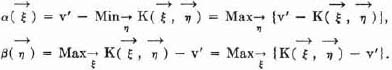
¹ I.e. we mean by loss the value of the play minus the actual outcome: for player 1 and (–v′) – (–K(, )) = K(, ) – v′ for player 2.

² Indeed, using the previous footnote and (17:13:a), (17:13:b)

I.e. each is a maximum loss.

³ Proof: It suffices to show this for ; the proof for is analogous.

Let be permanently optimal. Choose a * which is optimal against , i.e. with

By definition

Thus *, is a saddle point of K(, ) and therefore belongs to —i.e. it is good—by (l7:C:f) in 17.8.2.

¹ Cf. 17.1. Any other probabilities would lead to losses when “found out.” Cf. below.

² This is = {1, 0} or [1, 0, 0], respectively.

³ This is = [0, 1] or [0, 1, 0], respectively.

⁴ I.e. the bad strategy of “heads” (or “stone”) can be defeated only by “tails” (or “paper”), which is just as bad in itself.

⁵ Thus Chess and Backgammon are included.

⁶ The preceding discussion applies rather to the failure to “bluff.” Cf. 19.2. and 19.10.3.

¹ For a matrix (τ₁, τ₂) or for the corresponding bilinear form K(, ) symmetry is defined by

or equivalently by

It is remarkable that symmetry of the game Γ is equivalent to skew-symmetry, and not to symmetry, of its matrix or bilinear form.

² Thus skew-symmetry means that a reflection of the matrix scheme of Fig. 15 in 14.1.3. on its main diagonal (consisting of the fields (1, 1), (2, 2), etc.) carries it into its own negative. (Symmetry, in the sense of the preceding footnote, would mean that it carries it into itself.)

Now the matrix scheme of Fig. 15 is rectangular; it has β₂ columns and β₁ rows. In the case under consideration its shape must be unaltered by this reflection. Hence it must be quadratic,—i.e. β₁ = β₂. This is so, however, automatically, since the players 1, 2 are assumed to have the same role in Γ.

³ This is, of course, due to our knowing that . Without this—i.e. without the general theorem (16:F) of 16.4.3.—we should assert for the only the same which we obtained above for the v₁, v₂: and since

⁴ The players 1 and 2 have different roles in Matching Pennies: 1 tries to match, and 2 tries to avoid matching. Of course, one has a feeling that this difference is inessential and that the fairness of Matching Pennies is due to this inessentiality of the assymetry. This could be elaborated upon, but we do not wish to do this on this occasion. A better example of fairness without symmetry would be given by a game which is grossly unsymmetric, but in which the advantages and disadvantages of each player are so judiciously adjusted that a fair game—i.e. value v′ = 0—results.

A not altogether successful attempt at such a game is the ordinary way of “Rolling Dice.” In this game player 1—the “player”—rolls two dice, each of which bear the numbers 1, · · · , 6. Thus at each roll any total 2, · · · , 12 may result. These totals have the following probabilities:

The rule is that if the “player” rolls 7 or 11 (“natural”) he wins. If he rolls 2, 3, or 12 he loses. If he rolls anything else (4, 5, 6, or 8, 9, 10) then he rolls again until he rolls either a repeat of the original one (in which case he wins), or a 7 (in which case he loses). Player 2 (the “house”) has no influence on the play.

In spite of the great differences of the rules as they affect players 1 and 2 (the “player” and the “house”) their chances are nearly equal: A simple computation, which we do not detail, shows that the “player” has 244 chances against 251 for the “house,” out of a total of 495; i.e. the value of a play—played for a unit stake—is

Thus the approximation to fairness is reasonably good, and it may be questioned whether more was intended.

¹ I.e. secure himself a gain 0.