12.2Business Function Library

The Business Function Library (BFL) provides a range of specific business functions mainly from the internal cash flow statement. Table 12.1 contains some examples of calculations that are implemented in the BFL.

Function	Corresponding Database Procedure
Annual Depreciation	AFLBFL_DBDEPRECIATION_PROC AFLBFL_SLDEPRECIATION_PROC AFLBFL_SOYDEPRECIATION_PROC
Internal Rate of Return	AFLBFL_INTERNALRATE_PROC
Rolling Forecast	AFLBFL_FORECAST_PROC

Table 12.1Some Functions of the Business Function Library

The underlying algorithms and data models are quite extensive, and it’s beyond the scope of this book to introduce them in detail. In addition to calculations based on a fixed process, the BFL also exposes specific mathematical functions that are used within complex algorithms but can also be called independently.

For example, AFLBFL_LINEARAVERAGE_PROC is such a function, which can be used to determine a weighted average. The individual variables are weighted differently here compared to the standard arithmetic average. You can, for example, let values from the recent past play a greater role in the result than older values, which can be useful for some forecasts.

The following is the mathematical definition of the weighted average of the numeric values x1 to xn with the corresponding weights w1 to wn:

(w1 × x1 + … + wn × xn) ÷ (w1 + … + wn)

Let’s take as an example the seat utilization of flights of a fixed flight connection with sample data from Table 12.2.

Period	Year	Average Use (Percent)
1	2012	87.5%
2	2013	95%
3	2014	91%
4	2015	60%

Table 12.2Sample Data for Weighted Average

We use the period as a weighting factor and thus get the following weighted average:

(1 × 0.875 + 2 × 0.95 + 3 × 0.91 + 4 × 0.6) ÷ (1 + 2 + 3 + 4) = 0.7905 ~ 79 %

The normal average is approximately 83%. The lower value is due to the low utilization during the past year, which has more of an impact on the weighted average. The interface of the AFLBFL_LINEARAVERAGE_PROC function has the structure shown in Table 12.3.

Parameter	Explanation	Column Structure (Name, Type)
Input: Database table	Original data	VALUE	DOUBLE
Output: Result	In row N, the weighted average of the values up to the period N	AVERAGED_RESULT	DOUBLE

Table 12.3Interface of the LINEAR_AVERAGE Function from the BFL

As an application example, we want to use this function to determine the weighted average of seat utilization for all flights of one airline. The result should be a time-based progression over the years, which can provide a better data basis for a flight-utilization forecast than the normal calculation of the average because the current data are valued higher than results of the past. To determine the required values, we use the ZA4H_SEAT_UTIL CDS view as the data source from Listing 12.1. We determine the percentage utilization using a calculated field (utilization). Here, we consider the economy, business, and first class seats and convert the result to an ABAP floating-point number (abap.fltp), which corresponds to the SQL type DOUBLE.

@AbapCatalog.sqlViewName: 'ZA4H_SEAT_UTIL'
@EndUserText.label: 'CDS Views in Chapter 12'
define view Za4h_Cds_Seat as select from sflight {
carrid,
fldate,
case
when seatsmax = 0 then 0
else ( cast ( ( seatsocc + seatsocc_b + seatsocc_f )
as abap.fltp ) )
/ ( cast ( ( seatsmax + seatsmax_b + seatsmax_f )
as abap.fltp ) )
end as utilization
}

Listing 12.1CDS View for Determining the Seat Utilization

Now we create an ABAP Managed Database Procedure (AMDP), to which we transfer the current client and the airline as inputs; as outputs, we expect a table with the normal and the weighted average of seat utilization for all years for which data are available in the system. In Listing 12.2, you see the SQLScript implementation for calling the AFLBFL_LINEARAVERAGE_PROC BFL function. We first select the average seat utilization using the CDS view grouped by year that we defined previously, and thus call the BFL function. Finally, we use the calculation engine (CE) plan operator CE_VERTICAL_UNION (see Chapter 4, Section 4.2.2) to transfer the columns of the two internal tables to the result structure. The result of the calculation is displayed in Figure 12.2.

CLASS zcl_a4h_chapter12_linavg DEFINITION
PUBLIC
CREATE PUBLIC .

PUBLIC SECTION.
INTERFACES: if_amdp_marker_hdb.

TYPES: BEGIN OF ty_utilization,
year TYPE i,
average TYPE p LENGTH 4 DECIMALS 2,
linear_average TYPE p LENGTH 4 DECIMALS 2,
END OF ty_utilization.
TYPES tt_utilization TYPE TABLE OF ty_utilization.

METHODS: linear_average_utilization
IMPORTING
VALUE(iv_mandt) TYPE mandt
VALUE(iv_carrid) TYPE s_carrid
EXPORTING
VALUE(et_utilization) TYPE tt_utilization.

PROTECTED SECTION.
PRIVATE SECTION.
ENDCLASS.

CLASS zcl_a4h_chapter12_linavg IMPLEMENTATION.

METHOD linear_average_utilization BY DATABASE
PROCEDURE FOR HDB LANGUAGE SQLSCRIPT OPTIONS READ-ONLY
USING ZA4H_SEAT_UTIL.

lt_data = select 100 * to_double(avg(utilization))
as "VALUE", year(fldate) as "YEAR"
from ZA4H_SEAT_UTIL
where mandt = :iv_mandt and carrid = :iv_carrid
group by year(fldate);

call _SYS_AFL.AFLBFL_LINEARAVERAGE_PROC(:lt_data,:lt_avg );

et_utilization = CE_VERTICAL_UNION(
:lt_data, [ "YEAR", "VALUE" as "AVERAGE"],
:lt_avg, [ "AVERAGED_RESULT" as "LINEAR_AVERAGE"]);

ENDMETHOD.
ENDCLASS.

Listing 12.2ABAP Managed Database Procedure with Access to the BFL Function

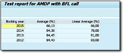
Figure 12.2Result of the Database Procedure in the ALV Table