The methods for the calculation of confidence intervals for a population mean and for differences between two population means for paired and unpaired samples were given in chapter 4. These methods are based on sample means, standard errors, and the t distribution and should strictly be used only for continuous data from Normal distributions (although small deviations from Normality are not important1). This is a so-called parametric approach as it essentially estimates the two parameters of the Normal distribution, that is, the mean and standard deviation.
For non-Normal continuous data the median of the population or the sample is often preferable to the mean as a measure of location. This chapter describes methods of calculating confidence intervals for a population median (the 50% quantile) or for other population quantiles from a sample of observations. Calculations of confidence intervals for the difference between two population medians (a non-parametric approach rather than the parametric approach mentioned above) for both unpaired and paired samples are described.
It is a common misapprehension that non-parametric methods are to be preferred if the sample size is small, since distributional assumption cannot be checked in these circumstances. However, non-parametric methods involve a loss of statistical power if Normality assumptions do hold, and so if the sample size is small and if there is good external evidence that the distributions are likely to be of the Normal form, the parametric methods may be preferred.
Because of the discrete nature of some of the sampling distributions involved in non-parametric analyses it is not usually possible to calculate confidence intervals with exactly the desired level of confidence. Hence, if a 95% confidence interval is wanted the choice is between the lowest possible level of confidence over 95% (a “conservative” interval) and the highest possible under 95%. There is no firm policy on which of these is preferred, but we shall mainly describe conservative intervals in this chapter. The exact level of confidence associated with any particular approximate level can be calculated from the distribution of the statistic being used although this may not be very straightforward. Further aspects of conservative and exact confidence intervals are given in chapter 13.
The methods outlined for obtaining confidence intervals are described in more detail in some textbooks on non-parametric statistics (for example, by Conover2). If there are many “ties” in the data, that is, observations with the same numerical value, then modifications to the formulae given here are needed.2 The calculations can be carried out using some statistical computer packages such as MINITAB.3
A confidence interval indicates the precision of the sample statistic as an estimate of the overall population value. Confidence intervals convey the effects of sampling variation but cannot control for non-sampling errors in study design or conduct. They should not be used for basic description of the sample data but only for indicating the uncertainty in sample estimates for population values of medians or other statistics.
The median, M, is defined as the value having half of the observations less than and half exceeding it. It is identified after first ranking the n sample observations in increasing order of magnitude. The sample median is used as an estimate of the population median. To find the 100(1 – α)% confidence interval for the population median first calculate the quantities

where Z1 – α/2 is the appropriate value from the standard Normal distribution for the 100(1 – α/2) percentile found in Table 18.1. Then round r and s to the nearest integers. The rth and sth observations in the ranking are the 100(1 — α)% confidence interval for the population median.
Worked example
For the data in the first example given in chapter 4 the median systolic blood pressure among 100 diabetic patients was M = 146 mmHg. Using the above formulae to calculate a 95% confidence interval gives

From the original data the 40th observation in increasing order is 142 mmHg and the 61st is 150 mmHg. The 95% confidence interval for the population median is thus from 142 to 150 mmHg.
This approximate method is satisfactory for most sample sizes.4 The exact method, based on the Binomial distribution, can be used instead for small samples, as shown in the example below, which uses Table 18.4.
Worked example
The results of a study measuring β-endorphin concentrations in pmol/l in n = 11 subjects who had collapsed while running in a half marathon5 were (in order of increasing value):

The sample median is the 6th observation in this ranking, that is M = 107·6 pmol/l. To find a confidence interval for the population median we use the Binomial distribution1 with n = 11 and probability π = 0·5. For a conservative 95% confidence interval we first find the largest X, which can take the values 0, 1, 2, …, 11 which gives the closest cumulative probability under 0·025 and the smallest X which gives the closest cumulative probability over 0·975. This can be done either by direct calculation or from tables.2 This gives Prob (X ≤ 1) = 0·006 and Prob (X ≤ 9) = 0·994.
The approximate 95% confidence interval is then found by the ranked observations that are one greater than those associated with the two probabilities, that is, the 2nd and 10th observations, giving 71·2 to 177·0 pmol/l.
The actual probability associated with this confidence interval is in fact 0·994 – 0·006 = 0·988 rather than 0·95, so effectively it is a 98·8% confidence interval. For sample sizes up to 100, the required rankings for approximate 90%, 95%, and 99% confidence intervals and associated exact levels of confidence are given directly in Table 18.4.
Alternatively, a non-conservative approximate 95% confidence interval can be found by calculating the smallest cumulative probability over 0·025 and the largest under 0·975. In this case we find Prob (X ≤ 2) = 0·033 and Prob (X ≤ 8) = 0·967, which give a 0·967 – 0·033 = 0·935 or 93·5% confidence interval from the 3rd to the 9th ranked observations, that is, from 83·0 to 160·0 pmol/l.
In this case the coverage probability of 93·5% is nearer to 95% than for the conservative interval coverage of 98·8%.
For this example the approximate large sample method gives a similar result as the conservative 95% confidence interval.
As another alternative, if the population distribution from which the observations came can be assumed to be symmetrical (but not of the Normal distribution shape) rather than skewed around the median, then the method described below in the section “Two samples: paired case” can be used, replacing the differences di given there by the sample observations.
A similar approach can be used to calculate confidence intervals for quantiles other than the median—for example, the 90th percentile, which divides the lower nine tenths from the upper tenth of the observations. For the qth quantile (q = 0·9 for the 90th percentile) r and s above are replaced by rq and sq given by

and

In finding confidence intervals for population differences between medians it is assumed that the data come from distributions that are identical in shape and differ only in location. Because of this assumption the non-parametric confidence intervals described below can be regarded as being either for the difference between the two medians, or the difference between the two means, or the difference between any other two measures of location such as a particular percentile. This assumption is not necessary for a valid test of the null hypothesis of no difference in population distributions but if it is not satisfied the interpretation of a statistically significant result is difficult.
Suppose x1, x2, …, xn1 represent the n1 observations in a sample from one population and y1, y2, …, yn2 the n2 observations on the same variable in a sample from a second population, where both sets of data are thought not to come from Normal distributions. The difference between the two population medians is estimated by the median of all the possible n1 × n2 differences xi – yj (for i = 1 to n1 and j = 1 to n2).
The confidence interval for the difference between the two population medians or means is also derived through these n1 × n2 differences.2 For an approximate 100(1 – α)% confidence interval first calculate

where Wα/2 is the 100α/2 percentile of the distribution of the Mann–Whitney test statistic.2 The Kth smallest to the Kth largest of the n1 × n2 differences then determine the 100(1 – α)% confidence interval. Values of K for finding approximate 90%, 95%, and 99% confidence intervals (α = 0·10, 0·05, and 0·01 respectively), together with the associated exact levels of confidence, for sample sizes of up to 25 are given directly in Table 18.5.
For studies where each sample size is greater than about 25, special tables are not required and K can be calculated approximately2 as

rounded up to the next integer value, where z1 – α/2 is the appropriate value from the standard Normal distribution for the 100(1 – α/2) percentile.
Worked example
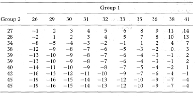
Consider the data in Table 5.1 on the globulin fraction of plasma (g/1) in two groups of 10 patients given by Swinscow.6 The computations are made easier if the data in each group are first ranked into increasing order of magnitude and then all the group 1 minus group 2 differences calculated as in Table 5.2. The estimate of the difference in population medians is now given by the median of these differences.
Table 5.1 Globulin fraction of plasma (g/1) in two groups of 10 patients6

Table 5.2 Differences in globulin fraction of plasma (g/1) between individuals in two groups of 10 patients6

From the 100 differences in Table 5.2 the 50th smallest difference is –6 g/1 and the 51st is –5 g/1, so the median difference is estimated as [–6 + (–5)]/2 = –5.5 g/1.
To calculate an approximate 95% confidence interval for the difference in population medians the value of K = 24 is found for n1 = 10, n2 = 10, and α = 0.05 from Table 18.5. The 24th smallest difference is –10 g/1 and the 24th largest is +1 g/1. The approximate 95% confidence interval (exact level 95·7%) for the difference in population medians or means is thus from –10 g/1 to +1 g/1.
Paired cases include, for example, studies of repeated measurements of the same variable on the same individuals over time and matched case-control comparisons. In these cases the paired differences are the observations of main interest. The method for finding confidence intervals described here assumes that, as well as the two distributions being identical except in location, the distribution of the paired differences is symmetrical. If this additional assumption seems unreasonable then the method described previously for a single sample can be applied to the paired differences.
Suppose that in a sample of size n the differences for each matched pair of measurements are d1, d2, …, dn. The difference between the two population medians is estimated by calculating all the n(n + 1)/2 possible averages of two of these differences taken together, including each difference with itself, and selecting their median.
The confidence interval for the difference between the population medians is also derived using these averaged differences. For an approximate 100(1 – α)% confidence interval first find the value of Wα/2 as the 100α/2 percentile of the distribution of the Wilcoxon one sample test statistic.2 Then if Wα/2 = K*, then the K*th smallest to the K*th largest of the averaged differences determine the 100(1 – α)% confidence interval. Values of K* for finding approximate 90%, 95%, and 99% confidence intervals (α = 0·10, 0·05, and 0·01), together with the associated exact levels of confidence, are given directly for sample sizes of up to 50 in Table 18.6. In general the coverage probability is only slightly higher than the specified one.
For sample sizes of about 50 or more, special tables are not required and K* can be calculated approximately2 as

rounded up to the next integer value, where z1 – α/2 is the appropriate value from the standard Normal distribution for the 100(1 – α/2) percentile.
Worked example
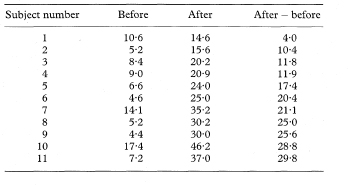
Consider further the β-endorphin concentrations in subjects running in a half marathon where 11 people were studied both before and after the event.5 The before and after concentrations (pmol/l) and their differences ordered by increasing size were as given in Table 5.3.
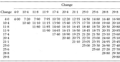
All the possible n(n + 1)/2 averages in this case where n = 11 give the 66 averages shown in Table 5.4. Thus, having found K* = 11 for n = 11 and α = 0·05 from Table 18.6, the 11 smallest averages are 4·00, 7·20, 7·90, 7·95, 10·40, 10·70, 11·10, 11·15, 11·80, 11·85, and 11·90; and the 11 largest averages are 25·10, 25·30, 25·45, 25·60, 26·90, 27·20, 27·40, 27·70, 28·80, 29·30, and 29·80. The approximate 95% (exact 95·8%) confidence interval for the difference between the population medians or means is thus given as 11·9 to 25·1 pmol/l around the sample median which is 18·8 pmol/l (the average of the 33rd and 34th ranked observations, 18·75 and 18·90, in the table of average differences). The triangular table of average differences helps to identify the required values, but a computer package such as MINITAB3 can rank the averages in order and select the appropriate ranked values.
Table 5.3 β-endorphin concentrations in 11 runners before and after a half marathon5

Table 5.4 Averages of differences in β-endorphin concentrations in 11 runners before and after a half marathon.5

The methods summarised above for the confidence intervals for differences between two medians can be applied to the difference between two means. However, this method would only be used when the means involved arise from a symmetric distribution which is not Normal such as a rectangular distribution.
A method for calculating confidence intervals for Spearman’s rank correlation coefficient, the non-parametric equivalent of the product moment correlation coefficient, is given in chapter 8.
It should be noted that there are differences of presentation in the tables referred to in Conover,2 Geigy scientific tables,7 and elsewhere. These result from the discrete nature of the distributions and whether7 or not2 the tabulated values are part of the critical region for the test of the null hypothesis. MINITAB3 uses large sample formulae with continuity corrections for computing the coverage probabilities of the confidence intervals for differences between medians even for sample sizes less than 20. This can lead to inaccuracies in the coverage probabilities given by the program. Alternative methods for calculating confidence intervals for medians, and differences in medians, based on the ‘bootstrap’ are given in chapter 13.
1 Bland M. An introduction to medical statistics. 2nd edn. Oxford: Oxford University Press, 1995: 89–92, 165–6.
2 Conover WJ. Practical non-parametric statistics. 2nd edn. New York: John Wiley, 1980: table A3, 223–5, table A7, 288–90, table A13.
3 Ryan BF, Joiner BL, Rogosa D. Minitab handbook. 3rd edn. Boston: Duxbury Press, 1994.
4 Hill ID. 95% confidence limits for the median. J Statist Comput Simulation 1987;28:80–1.
5 Dale G, Fleetwood JA, Weddell A, Ellis RD, Sainsbury JRC. β-Endorphin: a factor in “fun run” collapse. BMJ 1987;294:1004.
6 Swinscow TDV. Statistics at square one. 9th edn. (Revised by MJ Campbell). London: BMJ Publishing Group, 1996: 92–9.
7 Lentner C, ed. Geigy scientific tables. Volume 2. 8th edn. Basle: Ciba-Geigy, 1982: 156–62, 163.